Getting to know R and RStudio

AEA2026

Ben Harrap

Hello

Hello

Your turn!

Who you are
Where you’ve come from
Prior experience with coding

Outline

Important context:

RStudio interface
Packages
Projects and folders

Coding in R

Key concepts
Good practices
Error messages

An example workflow

Summaries and tables
Data visualisation
Regression

Data wrangling

Common transformations

What you’ll come away with

A better understanding of the R ecosystem
Lots of code examples
Lots more questions
The knowledge to figure out how to answer them

Housekeeping

Toilets
Breaks
Please ask questions
I use they/them pronouns

General format will be

Concept
Explanation
Practice

Tip

These boxes will have links to more information

Important context

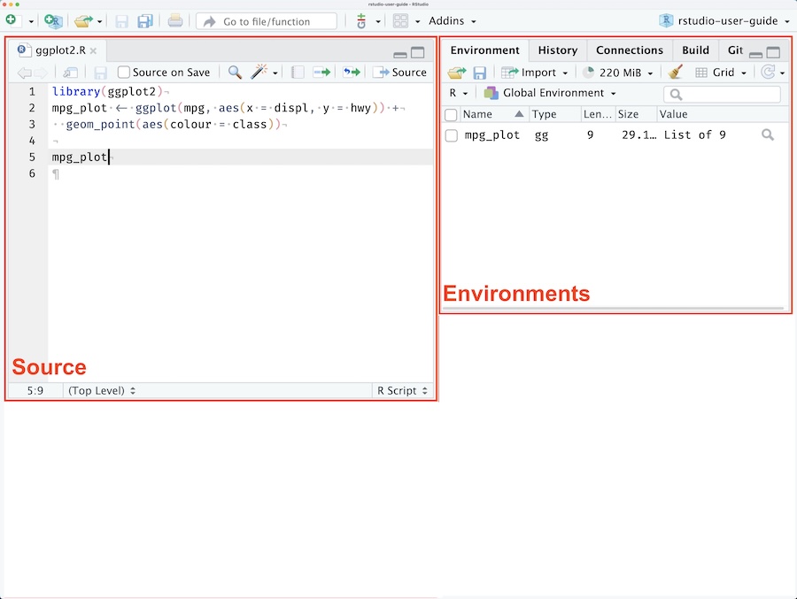
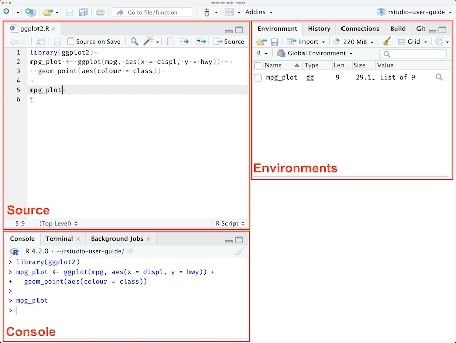
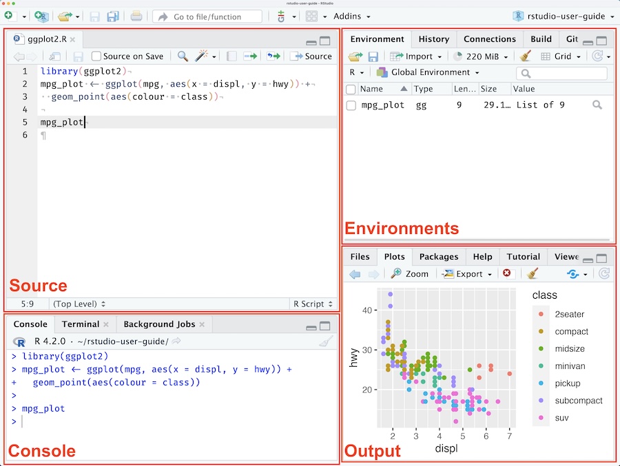
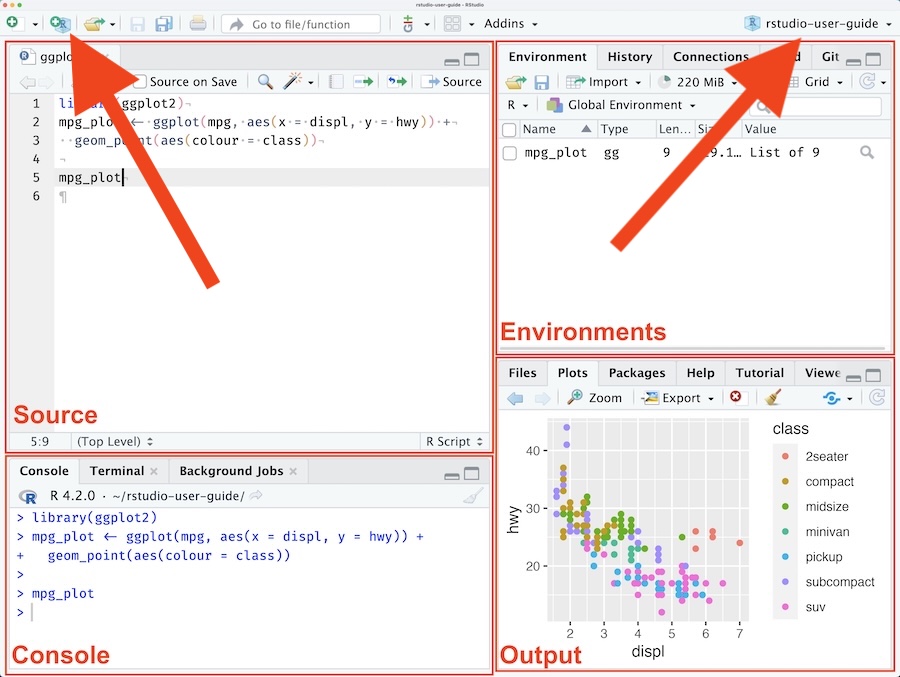
R vs. RStudio

R is the language that the code is written in.

RStudio is the interface (GUI) many people use to write R code in.

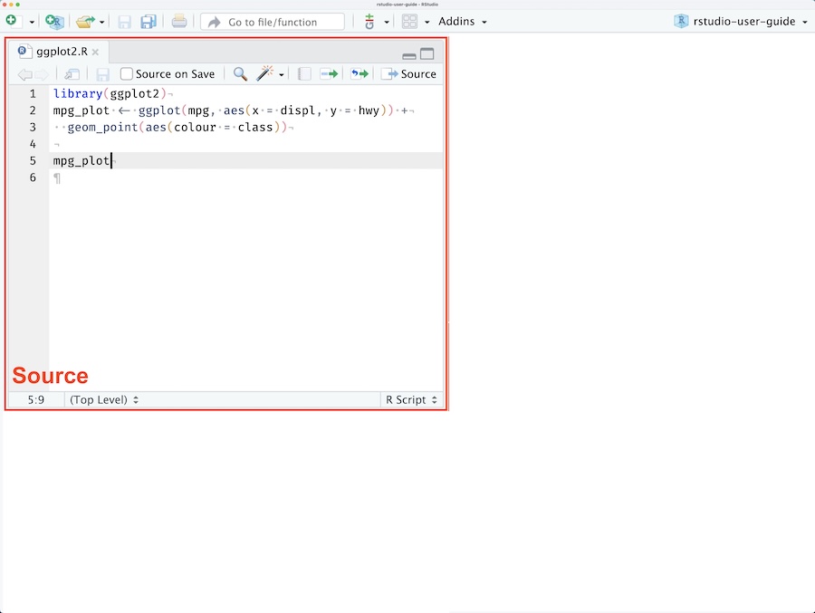
RStudio

`.RProj` files

Working directory

Reproducible workflows start with good file management:

Folders to organise your files
Descriptive names for files and folders
.RProj files set the working directory

2026-08-28-penguins-analysis.RProj
code/
  cleaning.R
  descriptives.R
  modelling.R
  visualisation.R
data/
  data_raw.csv

documentation/
  data_analysis_plan.docx
  data_dictionary.csv
output/                     
  forest_plot.png
  model_summary.csv
  sample_description.csv
penguins_report.docx

Absolute vs. relative locations

Absolute file path for the cleaning.R script:

//Volumes/shared drive/research/penguins/2026-08-28-penguins-analysis/code/cleaning.R

Relative file is relative to the current working directory:

code/cleaning.R

2026-08-28-penguins-analysis.RProj
code/
  cleaning.R
  descriptives.R
  modelling.R
  visualisation.R
data/
  data_raw.csv

documentation/
  data_analysis_plan.docx
  data_dictionary.csv
output/                     
  forest_plot.png
  model_summary.csv
  sample_description.csv
penguins_report.docx

Absolute vs. relative locations

Use .. to specify a folder ‘up’ from the working directory

So if the working directory is:

//Volumes/shared drive/research/penguins/2026-08-28-penguins-analysis

Then ../ would be

//Volumes/shared drive/research/penguins/

2026-08-28-penguins-analysis.RProj
code/
  cleaning.R
  descriptives.R
  modelling.R
  visualisation.R
data/
  data_raw.csv

documentation/
  data_analysis_plan.docx
  data_dictionary.csv
output/                     
  forest_plot.png
  model_summary.csv
  sample_description.csv
penguins_report.docx

Packages

A package is a collection of functions usually written around a particular goal or task.

To install a package, use the install.packages function

install.packages("tidyverse")

You then have to load the package using library()

library(tidyverse)

Tip

Once you install a package it’s available for any project, no need to install for every project.

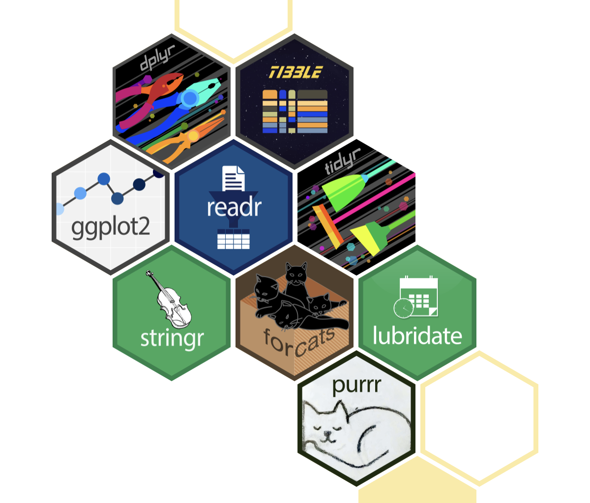
The `tidyverse`

A set of user-friendly tools for data manipulation and analysis

Reading in data (readr, readxl, haven, googlesheets4)
Data cleaning and manipulation (dplyr, tidyr, tibble)
Data visualisation (ggplot2)
Working with specific data types:
- Strings (stringr)
- Dates (lubridate)
- Factors (forcats)

Tip

See https://tidyverse.org/packages/ for details on what’s included in the tidyverse

Package conflicts

When you load packages that have the same function name, only one will take precedence

library(MASS)


Attaching package: 'MASS'

The following object is masked from 'package:dplyr':

    select

Prevent hours of debugging by being declarative!

Inline solution
Package solution

One option is to use two colons :: to declare the package as well as the function

data |> 
  dplyr::select()

The other option is to use the conflicted package and declare preferences upfront

library(conflicted)
conflicts_prefer(
  dplyr::select,
  dplyr::filter
  )

Question time

Let’s practice!

Install the tidyverse package

install.packages("tidyverse")

Load the tidyverse package

library(tidyverse)

Install the conflicted and MASS packages

install.packages(c("conflicted", "MASS"))

Load the MASS library to see the conflict warning

library(MASS)

Load the conflicted library and set the preferred package for select

library(conflicted)
conflicts_prefer(dplyr::select)

Coding in R

`penguins`

Our dataset for today — the built in dataset penguins

summary(penguins)

      species          island       bill_len        bill_dep    
 Adelie   :152   Biscoe   :168   Min.   :32.10   Min.   :13.10  
 Chinstrap: 68   Dream    :124   1st Qu.:39.23   1st Qu.:15.60  
 Gentoo   :124   Torgersen: 52   Median :44.45   Median :17.30  
                                 Mean   :43.92   Mean   :17.15  
                                 3rd Qu.:48.50   3rd Qu.:18.70  
                                 Max.   :59.60   Max.   :21.50  
                                 NAs    :2       NAs    :2      
  flipper_len      body_mass        sex           year     
 Min.   :172.0   Min.   :2700   female:165   Min.   :2007  
 1st Qu.:190.0   1st Qu.:3550   male  :168   1st Qu.:2007  
 Median :197.0   Median :4050   NAs   : 11   Median :2008  
 Mean   :200.9   Mean   :4202                Mean   :2008  
 3rd Qu.:213.0   3rd Qu.:4750                3rd Qu.:2009  
 Max.   :231.0   Max.   :6300                Max.   :2009  
 NAs    :2       NAs    :2

head(penguins, n = 4)

  species    island bill_len bill_dep flipper_len body_mass    sex year
1  Adelie Torgersen     39.1     18.7         181      3750   male 2007
2  Adelie Torgersen     39.5     17.4         186      3800 female 2007
3  Adelie Torgersen     40.3     18.0         195      3250 female 2007
4  Adelie Torgersen       NA       NA          NA        NA   <NA> 2007

Comments

#### This is a bookmark ####
# This is a comment, below is code
data |>
  select(species, island)

Use comments explain context, intention, functionality etc.

Use bookmarks to navigate sections of code

#### Level 1 ####

##### Level 2 ######

###### Level 3 ######

Elements of code

There are different terms for different elements of code

data |>
  select(
    species,
    island
  )

In the above code:

data is an object
select is a function
species and island are arguments of the select function

Assignment (`<-`)

R prints results in the console by default

read_csv("data/penguins.csv")

# A tibble: 344 × 8
   species island    bill_len bill_dep flipper_len body_mass sex     year
   <chr>   <chr>        <dbl>    <dbl>       <dbl>     <dbl> <chr>  <dbl>
 1 Adelie  Torgersen     39.1     18.7         181      3750 male    2007
 2 Adelie  Torgersen     39.5     17.4         186      3800 female  2007
 3 Adelie  Torgersen     40.3     18           195      3250 female  2007
 4 Adelie  Torgersen     NA       NA            NA        NA <NA>    2007
 5 Adelie  Torgersen     36.7     19.3         193      3450 female  2007
 6 Adelie  Torgersen     39.3     20.6         190      3650 male    2007
 7 Adelie  Torgersen     38.9     17.8         181      3625 female  2007
 8 Adelie  Torgersen     39.2     19.6         195      4675 male    2007
 9 Adelie  Torgersen     34.1     18.1         193      3475 <NA>    2007
10 Adelie  Torgersen     42       20.2         190      4250 <NA>    2007
# ℹ 334 more rows

Assign results using <- to store in an object

data <- read_csv("data/penguins.csv")

Tip

The shortcut for the assignment operator is Alt + - or Option + -

Accessing elements of an object

Sometimes we need to access one element of an object, such as a single column in our data

We can do this using $ or [""]

data$species

data["species"]

This is not always required, such as in the context of pipes

Pipes (`|>`)

Chain sequences of functions together using pipes

data <- read_csv("data/penguins.csv")
data <- filter(data, species == "Chinstrap")
data <- mutate(data,
               body_mass_kg = body_mass/1000)
summarise(data, mean_body_mass = mean(body_mass_kg))

Pipes effectively fill in the first argument of a function:

data <- read_csv("data/penguins.csv")
data |>
  filter(species == "Chinstrap") |>
  mutate(body_mass_kg = body_mass/1000) |>
  summarise(mean_body_mass = mean(body_mass_kg))

Tip

The shortcut for the pipe operator is Ctrl + Shift + M

Keyboard shortcuts

To see all keyboard shortcuts, click on ‘Keyboard Shortcuts Help’ in the ‘Help’ menu

My most commonly used are:

Insert pipe (Ctrl + Shift + M)
Insert assignment operator (Option/Alt + -)
Move line up or down (Option/Alt + Up/Down)
Duplicate line or selection (Cmd + Option + Up/Down)
Delete line or selection (Cmd + D)
Comment or uncomment (Cmd + Shift + C)

Common types of things

Numbers and integers
Logicals
Factors (https://forcats.tidyverse.org/)
Dates/times (https://lubridate.tidyverse.org/)
Characters (https://stringr.tidyverse.org/)
Missing
Vectors and lists
Data frames and tibbles (https://tibble.tidyverse.org/)

Missing

Missing has its own special identity in R — NA

penguin_species <- c("Adelie", "Gentoo", "Chinstrap", NA)
penguin_species

[1] "Adelie"    "Gentoo"    "Chinstrap" NA

It also has its own special function to check if something is missing:

is.na(penguin_species)

[1] FALSE FALSE FALSE  TRUE

Be sure to use is.na(), if you just use the equals operator it won’t work:

penguin_species == NA

[1] NA NA NA NA

data |> mutate(ldr=bill_len/bill_dep)

data |> mutate(ldr = bill_len / bill_dep)

data |> 
  mutate(
    ldr = bill_len / bill_dep
  )

data |> 
  mutate(
    length_depth_ratio = bill_len / bill_dep
  )

data |> 
  mutate(
    # Calculate the bill length/depth ratio
    length_depth_ratio = bill_len / bill_dep
  )

#### Cleaning ####
data |> 
  mutate(
    # Calculate the bill length/depth ratio
    length_depth_ratio = bill_len / bill_dep
  )

#### Plots ####
ggplot(
  ⋮

Tip

Formatters like air do a lot of the work for you https://tidyverse.org/blog/2025/02/air/

Common errors

Trailing comma
Missing comma
Equals signs
Unclosed bracket
Too many brackets

penguin_species <- c(
  "Adelie", 
  "Gentoo", 
  "Chinstrap",
  )

Error in `c()`:
! argument 4 is empty

penguin_species <- c(
  "Adelie"
  "Gentoo"
  "Chinstrap"
  )

Error in parse(text = input): <text>:3:3: unexpected string constant
2:   "Adelie"
3:   "Gentoo"
     ^

data |> 
  mutate(
    is_chinstrap = species = "Chinstrap"
  )

Error in parse(text = input): <text>:3:28: unexpected '='
2:   mutate(
3:     is_chinstrap = species =
                              ^

data |> 
  mutate(
    is_chinstrap = species == "Chinstrap"
    
ggplot(data)

Error in parse(text = input): <text>:5:1: unexpected symbol
4:     
5: ggplot
   ^

data |> 
  mutate(
    is_chinstrap = species == "Chinstrap"
  )
)

Error in parse(text = input): <text>:5:1: unexpected ')'
4:   )
5: )
   ^

Error messages

They try to tell you what the problem was, but it’s not always easy

Read the error message
Look at your code
Read help files
Check for cheatsheets
Web search
Join a community
Ask an LLM

Try to figure out the solution yourself before consulting an LLM, you’ll learn more!

Tip

You’ll get lots of error messages as you learn how to code, this is normal

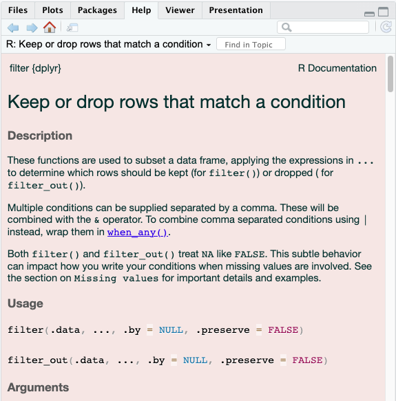
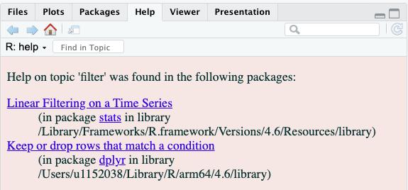
Help files

Documentation explaining how a function works:

Description
Arguments
Examples

Run ?filter from the console, or search the ‘Help’ pane

Let’s practice!

What might these error messages mean?

tidyverse

Error:
! object 'tidyverse' not found

library(tidyvers)

Error in `library()`:
! there is no package called 'tidyvers'

1 + "2"

Error in `1 + "2"`:
! non-numeric argument to binary operator

penguin_species <- c(
  "Adelie", 
  "Gentoo", 
  "Chinstrap",
  )

Error in `c()`:
! argument 4 is empty

penguin_species <- c(
  "Adelie", 
  "Gentoo", 
  "Chinstrap",
  King
  )

Error:
! object 'King' not found

Question time

Break time!

Example workflow

Continuing with the penguins dataset, we’ll cover:

Summaries and tables
Data visualisation
Regression

Summaries and tables

`dplyr::summarise()`

The summarise() function applies the specified summary to the whole dataset

data |> 
  summarise(
    number_penguins = n(),
    mean_body_mass = mean(body_mass, na.rm = TRUE),
    .by = c(species, sex)
  )

# A tibble: 8 × 4
  species   sex    number_penguins mean_body_mass
  <chr>     <chr>            <int>          <dbl>
1 Adelie    male                73          4043.
2 Adelie    female              73          3369.
3 Adelie    <NA>                 6          3540 
4 Gentoo    female              58          4680.
5 Gentoo    male                61          5485.
6 Gentoo    <NA>                 5          4588.
7 Chinstrap female              34          3527.
8 Chinstrap male                34          3939.

If .by is specified, it applies the summaries within each group
The summary is returned in the same format as the input (data frame, tibble)

`janitor::tabyl()`

The tabyl() function is a convenient way to tabulate data.

One variable

library(janitor)
data |> 
  tabyl(species)

   species   n   percent
    Adelie 152 0.4418605
 Chinstrap  68 0.1976744
    Gentoo 124 0.3604651

Two variables

data |> 
  tabyl(species, sex)

   species female male NA_
    Adelie     73   73   6
 Chinstrap     34   34   0
    Gentoo     58   61   5

When tabulating two variables, the first argument is for rows, the second argument is for columns
In both cases, the tabulation is returned as a data frame

`janitor::tabyl()`

There are several helper functions starting with adorn_*, that add to the tabulation

data |> 
  tabyl(species) |> 
  adorn_pct_formatting()

   species   n percent
    Adelie 152   44.2%
 Chinstrap  68   19.8%
    Gentoo 124   36.0%

For two variables, adorn_* functions sometimes need rows or columns specified

data |> 
  tabyl(species, sex) |> 
  adorn_totals("col") |> 
  adorn_percentages("row") |> 
  adorn_ns()

   species         female           male            NA_   Total
    Adelie 0.4802632 (73) 0.4802632 (73) 0.03947368 (6) 1 (152)
 Chinstrap 0.5000000 (34) 0.5000000 (34) 0.00000000 (0) 1  (68)
    Gentoo 0.4677419 (58) 0.4919355 (61) 0.04032258 (5) 1 (124)

`gtsummary`

The gtsummary package has many functions for producing summary tables

library(gtsummary)

We’ll focus on the tbl_summary() function

# Function arguments
tbl_summary(
  data,
  by = NULL,
  label = NULL,
  statistic = list(all_continuous() ~ "{median} ({p25}, {p75})", all_categorical() ~
    "{n} ({p}%)"),
  digits = NULL,
  type = NULL,
  value = NULL,
  missing = c("ifany", "no", "always"),
  missing_text = "Unknown",
  missing_stat = "{N_miss}",
  sort = all_categorical(FALSE) ~ "alphanumeric",
  percent = c("column", "row", "cell"),
  include = everything()
)

`tbl_summary()`

penguin_summary <- tbl_summary(
  data,
1  by = species,
2  include = c(
    sex,
    bill_len,
    flipper_len,
  )
)

1: Which variable to produce summaries by
2: Which variables to summarise

Characteristic	Adelie N = 152¹	Chinstrap N = 68¹	Gentoo N = 124¹
sex
female	73 (50%)	34 (50%)	58 (49%)
male	73 (50%)	34 (50%)	61 (51%)
Unknown	6	0	5
bill_len	38.8 (36.7, 40.8)	49.6 (46.3, 51.2)	47.3 (45.3, 49.6)
Unknown	1	0	1
flipper_len	190 (186, 195)	196 (191, 201)	216 (212, 221)
Unknown	1	0	1
¹ n (%); Median (Q1, Q3)

`tbl_summary()`

penguin_summary <- tbl_summary(
  data,
1  by = species,
2  include = c(
    sex,
    bill_len,
    flipper_len,
  ),
3  statistic = list(
    all_continuous() ~ "{mean} ({sd})",
    all_categorical() ~ "{n} [{p}%]"
  )
)

1: Which variable to produce summaries by
2: Which variables to summarise
3: What statistics to produce

Characteristic	Adelie N = 152¹	Chinstrap N = 68¹	Gentoo N = 124¹
sex
female	73 [50%]	34 [50%]	58 [49%]
male	73 [50%]	34 [50%]	61 [51%]
Unknown	6	0	5
bill_len	38.8 (2.7)	48.8 (3.3)	47.5 (3.1)
Unknown	1	0	1
flipper_len	190 (7)	196 (7)	217 (6)
Unknown	1	0	1
¹ n [%]; Mean (SD)

`tbl_summary()`

penguin_summary <- tbl_summary(
  data,
1  by = species,
2  include = c(
    sex,
    bill_len,
    flipper_len,
  ),
3  statistic = list(
    all_continuous() ~ "{mean} ({sd})",
    all_categorical() ~ "{n} [{p}%]"
  ),
4  label = list(
    sex = "Sex",
    bill_len = "Bill length",
    flipper_len = "Flipper length",
    body_mass = "Body mass (g)"
  )
)

1: Which variable to produce summaries by
2: Which variables to summarise
3: What statistics to produce
4: Specify labels for the variables

Characteristic	Adelie N = 152¹	Chinstrap N = 68¹	Gentoo N = 124¹
Sex
female	73 [50%]	34 [50%]	58 [49%]
male	73 [50%]	34 [50%]	61 [51%]
Unknown	6	0	5
Bill length	38.8 (2.7)	48.8 (3.3)	47.5 (3.1)
Unknown	1	0	1
Flipper length	190 (7)	196 (7)	217 (6)
Unknown	1	0	1
¹ n [%]; Mean (SD)

`tbl_summary()`

penguin_summary <- tbl_summary(
  data,
1  by = species,
2  include = c(
    sex,
    bill_len,
    flipper_len,
  ),
3  statistic = list(
    all_continuous() ~ "{mean} ({sd})",
    all_categorical() ~ "{n} [{p}%]"
  ),
4  label = list(
    sex = "Sex",
    bill_len = "Bill length",
    flipper_len = "Flipper length",
    body_mass = "Body mass (g)"
  ),
5  missing_text = "Missing",
  missing_stat = "{p_miss}"
)

1: Which variable to produce summaries by
2: Which variables to summarise
3: What statistics to produce
4: Specify labels for the variables
5: Control how missing data are summarised

Characteristic	Adelie N = 152¹	Chinstrap N = 68¹	Gentoo N = 124¹
Sex
female	73 [50%]	34 [50%]	58 [49%]
male	73 [50%]	34 [50%]	61 [51%]
Missing	3.9	0	4.0
Bill length	38.8 (2.7)	48.8 (3.3)	47.5 (3.1)
Missing	0.7	0	0.8
Flipper length	190 (7)	196 (7)	217 (6)
Missing	0.7	0	0.8
¹ n [%]; Mean (SD)

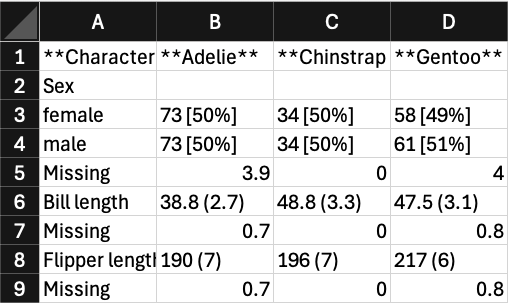
`tbl_summary()`

To save the output from tbl_summary(), we:

convert it to a tibble
save this as csv file

penguin_summary |> 
  as_tibble() |> 
  write_csv(
    "data/penguin_summary.csv",
    na = ""
    )

Other packages for tables

Creating tables via Quarto or RMarkdown:

flextable has the best MS Word support
kable is good for PDF output
gt is highly customisable for HTML output

These do not create summaries for you!

Let’s practice!

Use summarise() to calculate the median body mass within each penguin species

data |> 
  summarise(
    median_body_mass = median(body_mass, na.rm = TRUE),
    .by = species
  )

Use tabyl() to tabulate the number of species and total penguins counted in each year

data |> 
  tabyl(species, year) |> 
  adorn_totals("row")

Use tbl_summary() to summarise body mass and sex by island

tbl_summary(
  data,
    by = island,
  include = c(
    sex,
    body_mass, 
  )
)

Data visualisation

Package options

plot() — base R

ggplot2 — part of the tidyverse, highly customisable

tidyplots — simpler interface to ggplot2

`ggplot2`

There are many plot types available, including:

Raw data

Scatter plots (geom_point())
Dot plots (geom_dotplot())
Line graph (geom_line())

Summaries

Bar plots (geom_bar(), geom_col())
Bars with errors (geom_errorbar())
Box and whisker plots (geom_boxplot())

Distributions

Histogram (geom_hist())
Density (geom_density())
Violin (geom_violin())

Tip

See the documentation for all available plots https://ggplot2.tidyverse.org/reference/index.html

`ggplot2`

All plots start with the ggplot() function

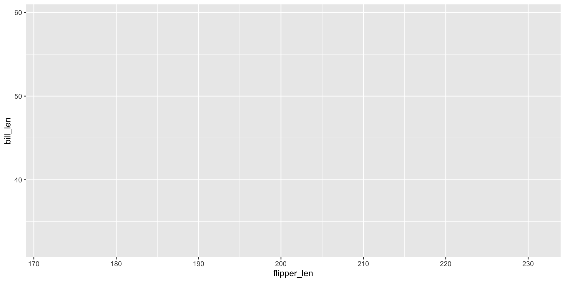
ggplot(
  data,
  aes(
    x = flipper_len,
    y = bill_len
  )
)

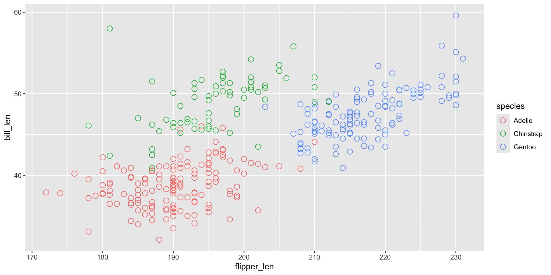
Scatter plot

From this, we add to the plot using the + symbol

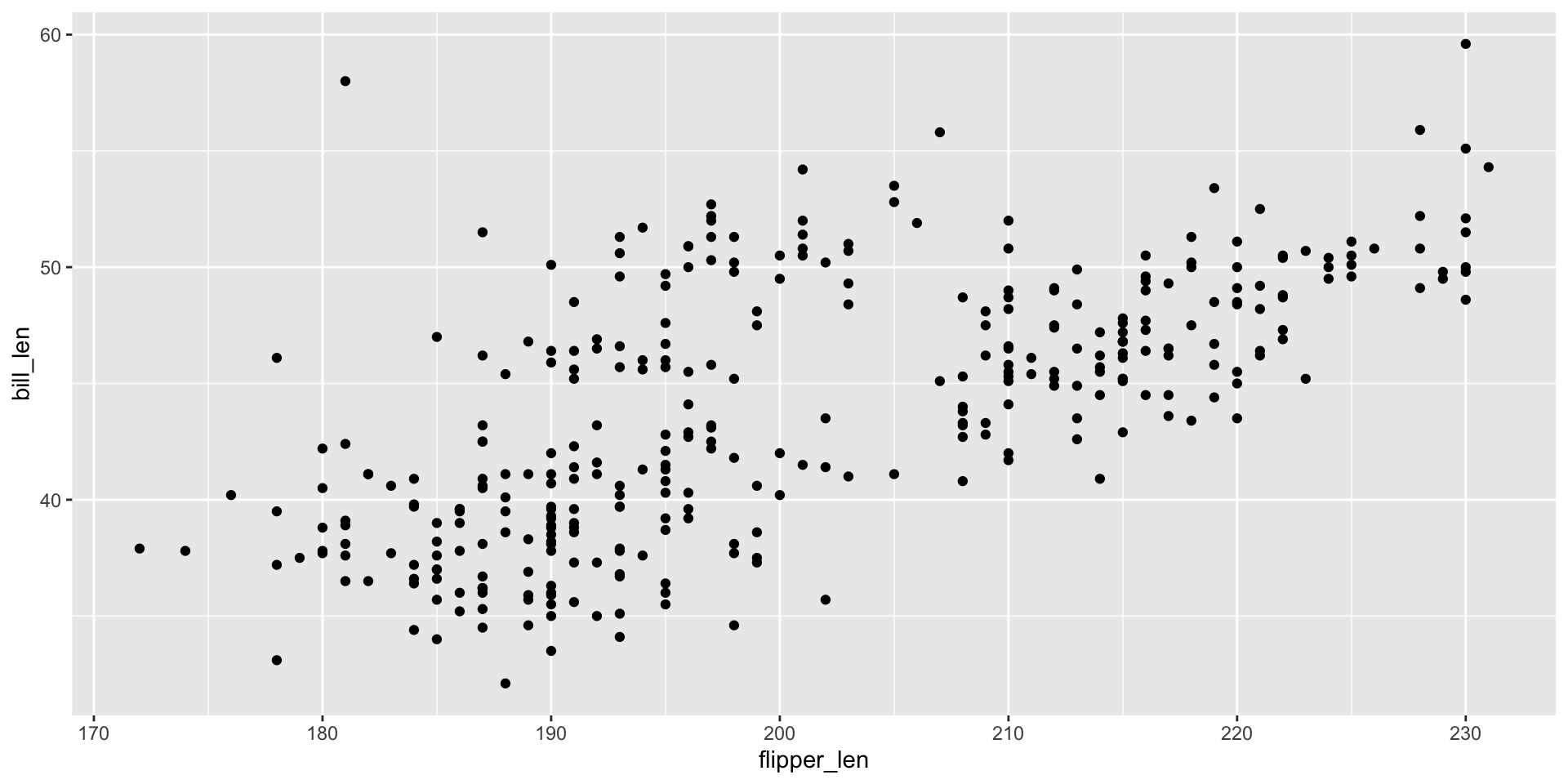
ggplot(
  data,
  aes(
    x = flipper_len,
    y = bill_len
  )
) +
  geom_point()

Bar plot

For some plots, it doesn’t make sense to plot the raw data.

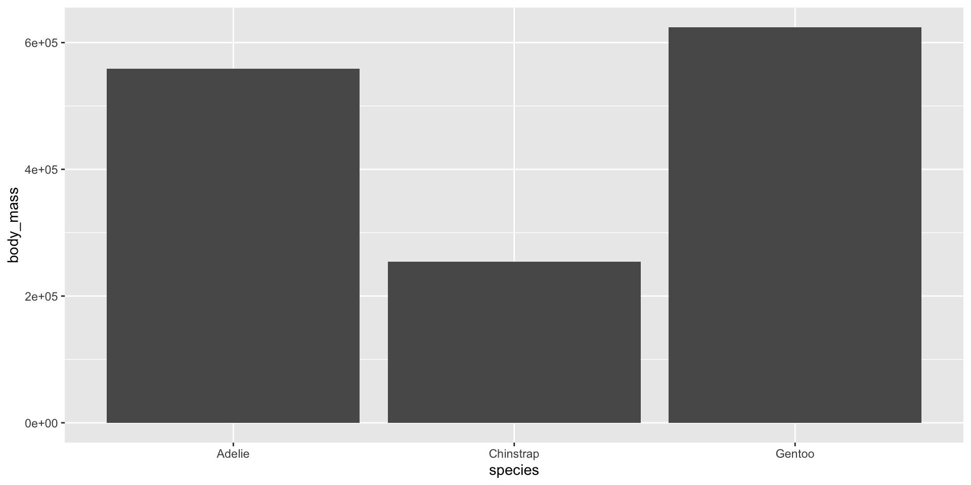
ggplot(
  data,
  aes(
    x = species,
    y = body_mass
  )
) +
  geom_col()

Tip

Use geom_col() on summarised data, geom_bar() to summarise raw data

Bar plot

Instead, we need to summarise the data first and plot the summarised values

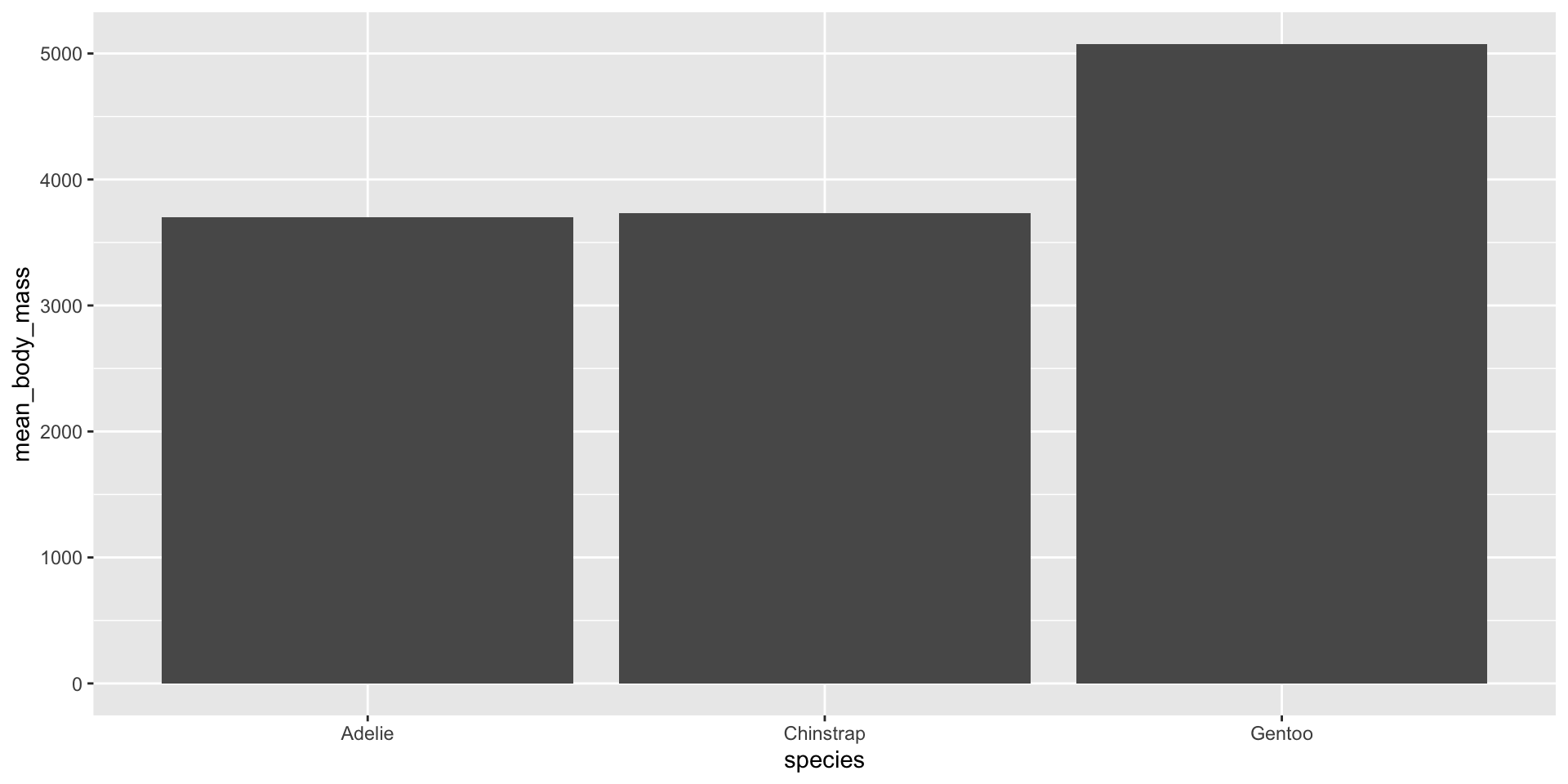
data |> 
  summarise(
    mean_body_mass = mean(body_mass, na.rm = T),
    .by = species
  ) |> 
  ggplot(
    aes(
      x = species,
      y = mean_body_mass
    )
  ) +
  geom_col()

Tip

Use geom_col() on summarised data, geom_bar() to summarise raw data

Line graph

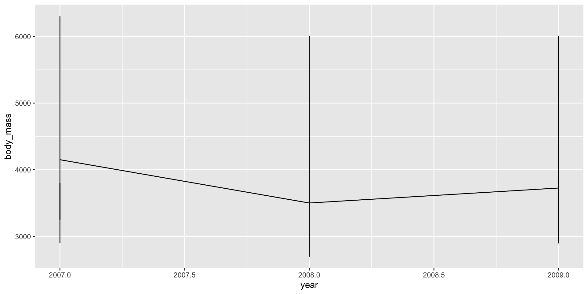
ggplot(
  data,
  aes(
    x = year,
    y = body_mass
  )
) +
geom_line()

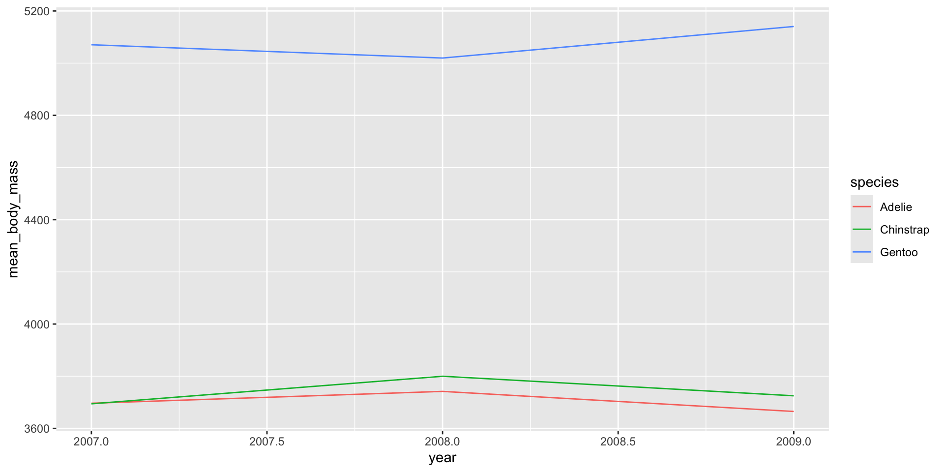
Line graph

data |>
  summarise(
    mean_body_mass = mean(body_mass, na.rm = T),
    .by = c(year, species)
  ) |>
  ggplot(
    aes(
      x = year,
      y = mean_body_mass,
      colour = species
    )
  ) +
  geom_line()

Questions?

Customising a plot

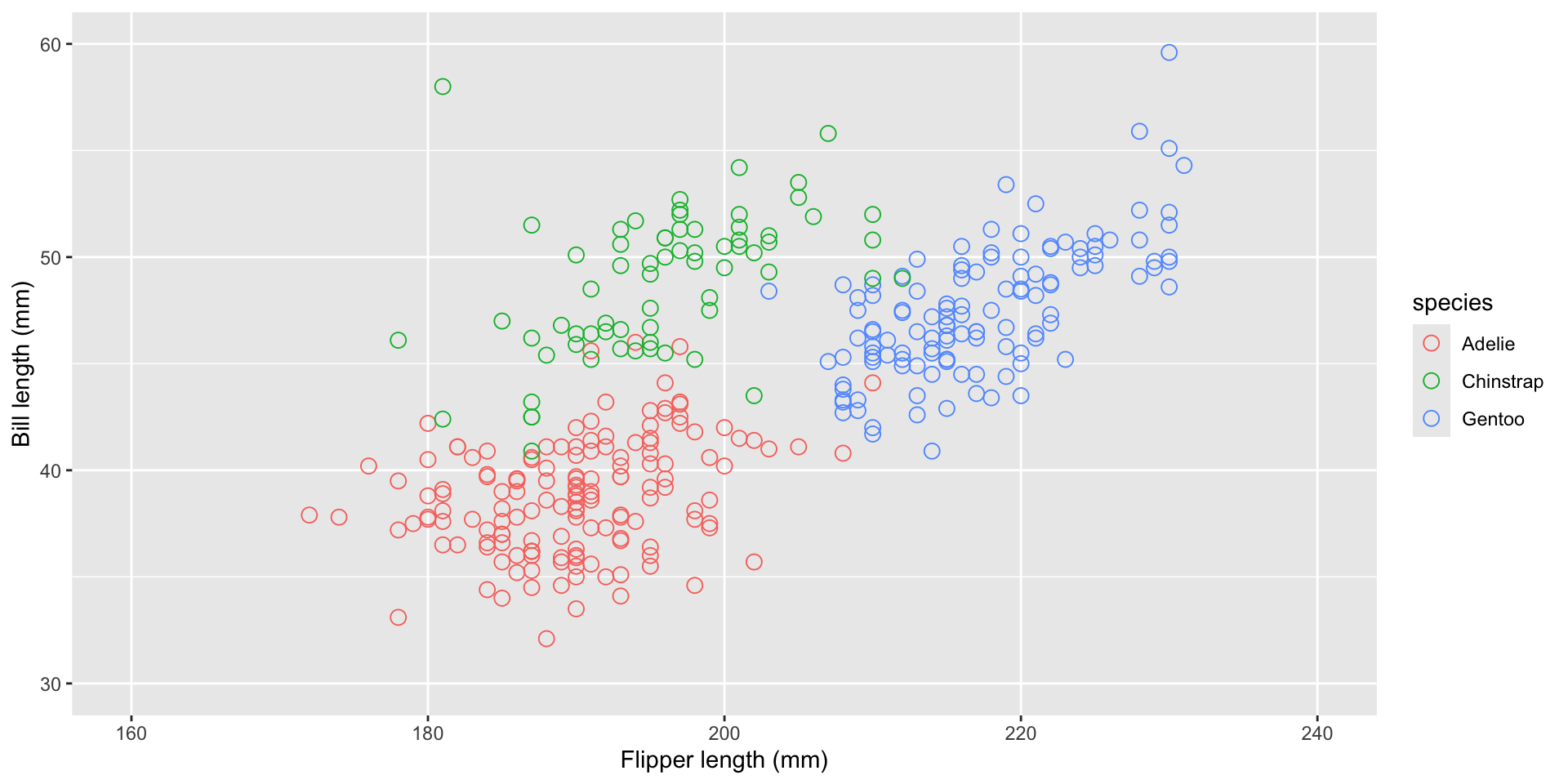
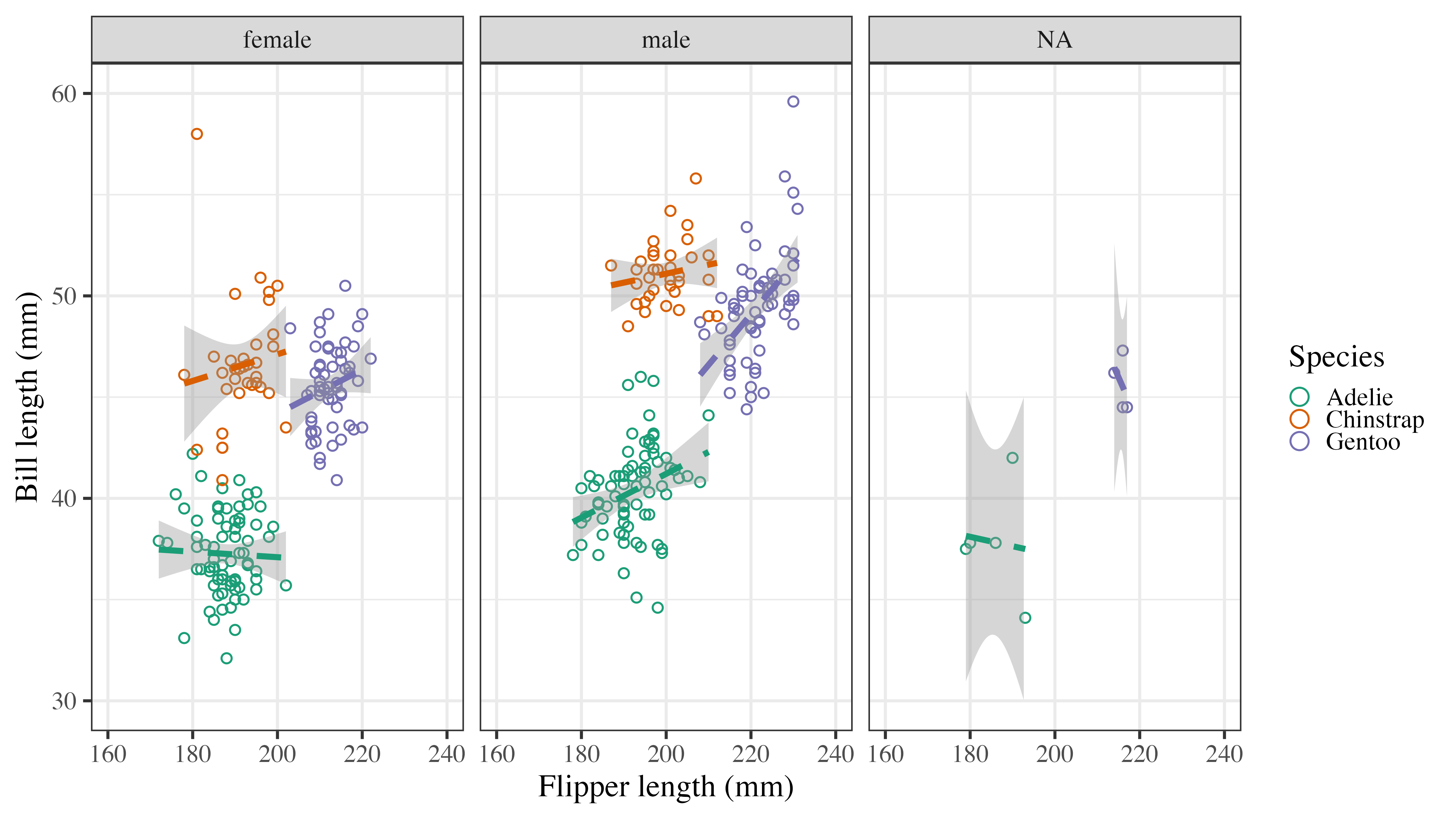
penguin_plot <- ggplot(
  data,
  aes(
    x = flipper_len,
    y = bill_len,
    colour = species
  )
) +
  geom_point(
    size = 3,
    shape = 1
    )

penguin_plot

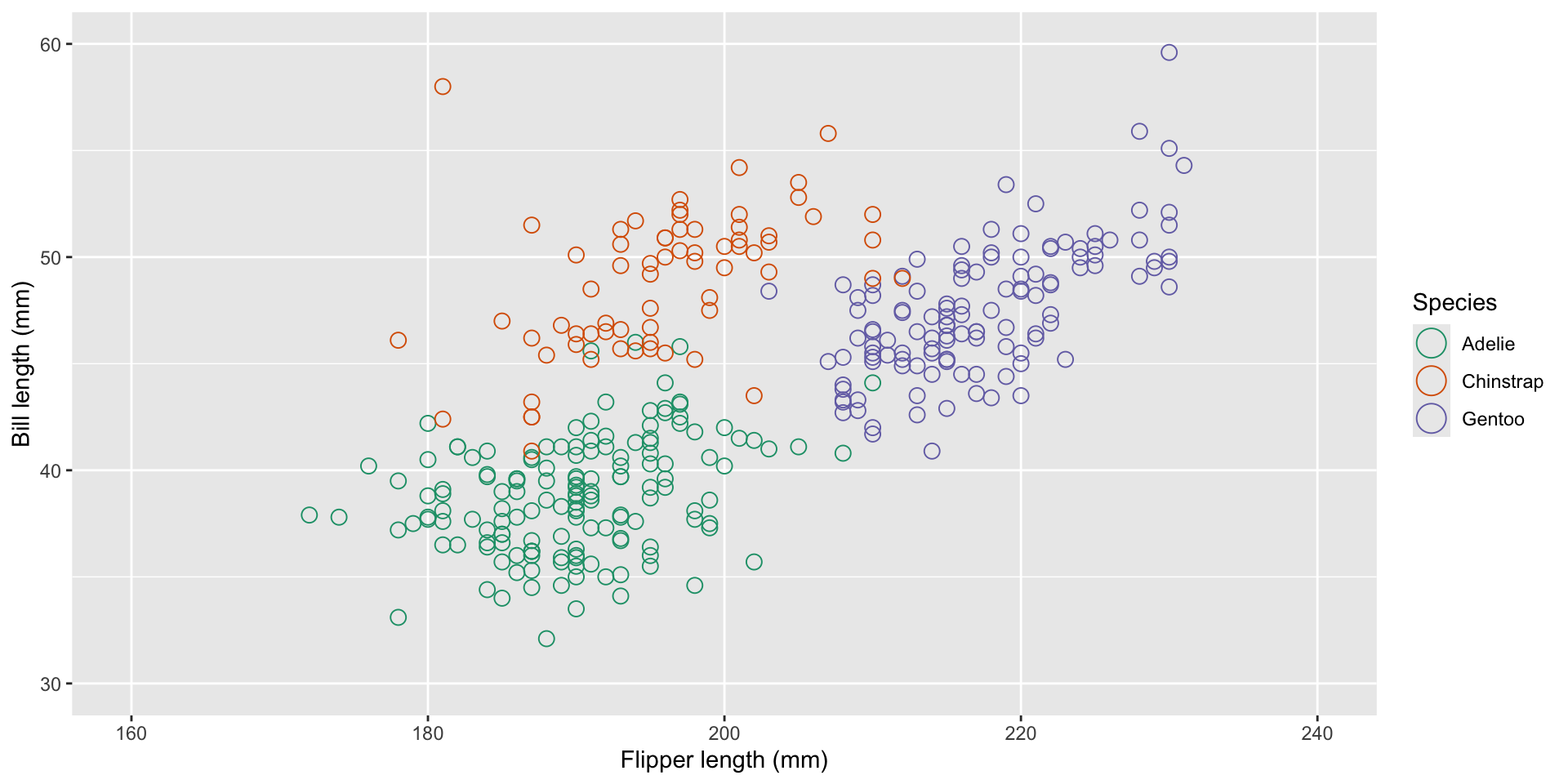
Customising axes

penguin_plot <- penguin_plot +
  scale_x_continuous(
    name = "Flipper length (mm)",
    limits = c(160, 240),
    breaks = seq(160,240,20),
    minor_breaks = NULL
  ) +
  scale_y_continuous(
    name = "Bill length (mm)",
    limits = c(30, 60),
    breaks = seq(30, 60, 10),
    minor_breaks = seq(35, 55, 10)
  ) 
penguin_plot

Customising the legend

penguin_plot <- penguin_plot + 
  scale_colour_manual(
    name = "Species",
    values = c("#1b9e77", "#d95f02", "#7570b3")
  ) +
  guides(color = guide_legend(override.aes = list(size = 6)))
penguin_plot

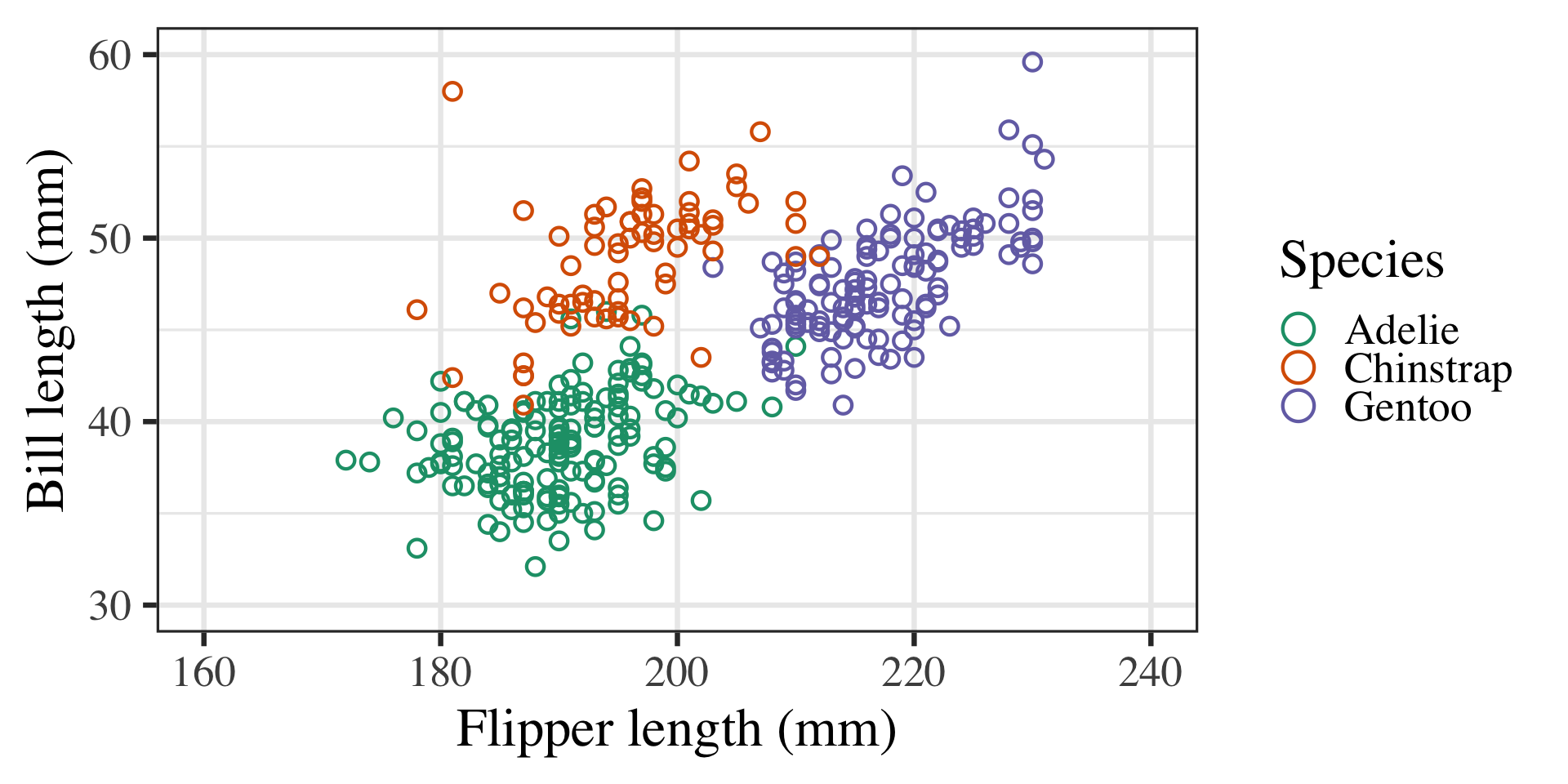
Customising with a theme

penguin_plot <- penguin_plot + 
  theme_bw(
    base_size = 25,
    base_family = "serif"
  )
penguin_plot

Tip

There are several themes available! theme_minimal() is popular, but has a transparent background.

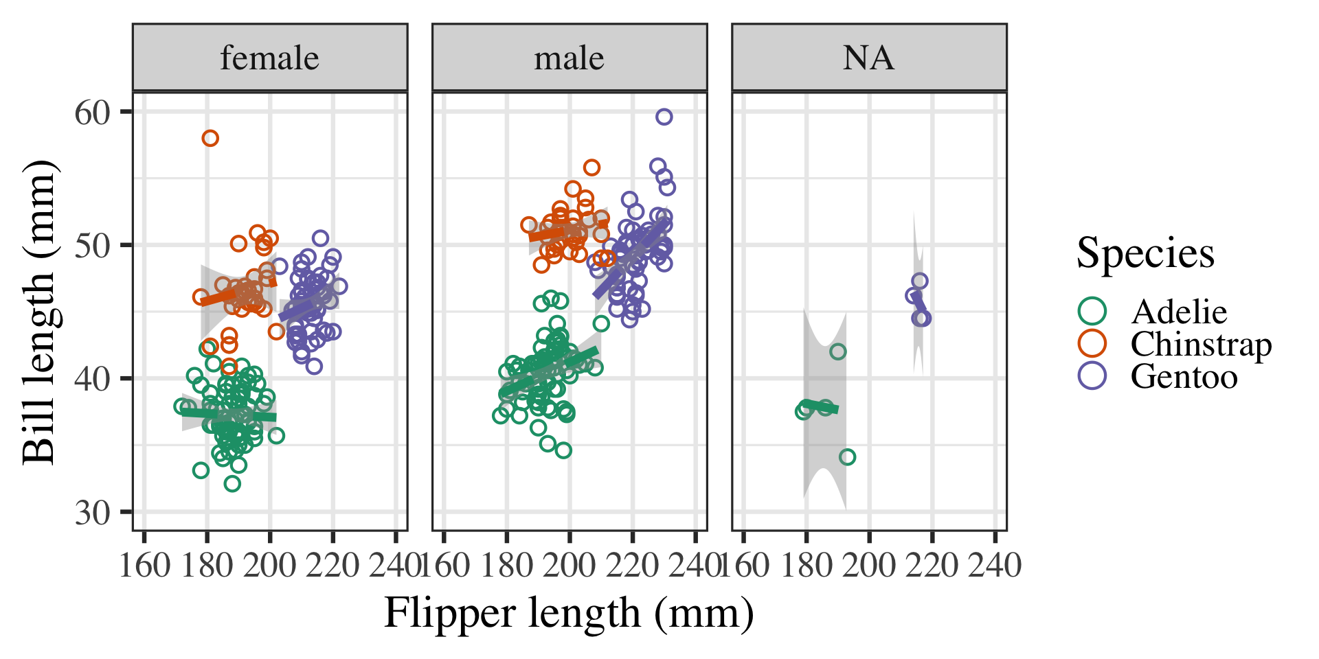
Adding an element

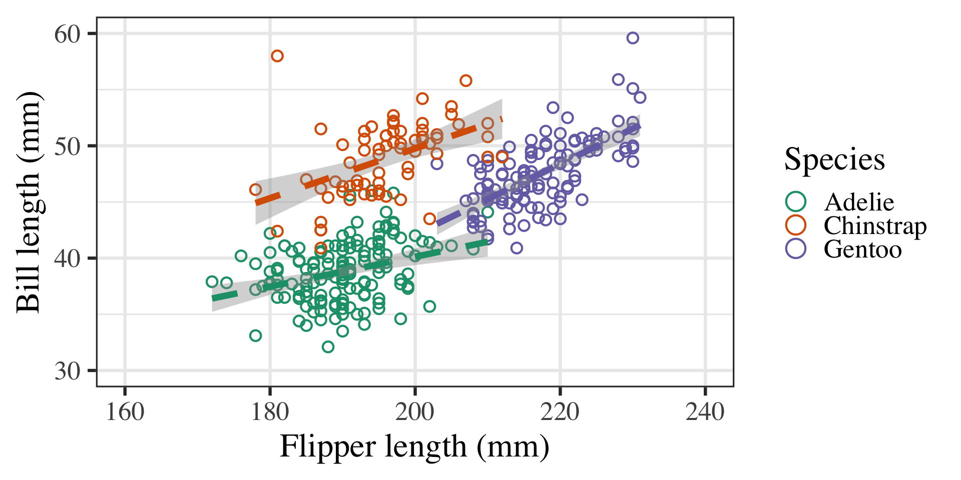
penguin_plot <- penguin_plot +
  geom_smooth(
    method = "lm",
    linetype = "dashed",
    show.legend = FALSE
  )
penguin_plot

Saving the output

ggsave(
  "img/penguin_plot.png",
  penguin_plot,
  width = 16,
  height = 9,
  units = "in",
)

Let’s practice!

Use ggplot2 to make a bar chart showing the count of each penguin species, format the axes, and add a theme.

Initial specification

practice_plot <- ggplot(
  data,
  aes(
    x = species
  )
)

Adding the bars

practice_plot <- practice_plot +
  geom_bar()

Format the axes

practice_plot <- practice_plot +
  scale_x_discrete(
    name = NULL
  ) +
  scale_y_continuous(
    name = "Count",
    limits = c(0, 160)
  )

Add a theme

practice_plot <- practice_plot +
  theme_bw()

Questions?

Regression

Model notation

To regress body_mass on sex and species, we write:

regression_results <- lm(
  body_mass ~ sex + species,
  data = data
)

Outcome (body_mass) left of the tilde ~

Covariates right of the tilde, separated with a plus +

# Function arguments
lm(
  formula, 
  data, 
  subset, 
  weights, 
  na.action,
  method = "qr",
  model = TRUE, 
  x = FALSE, 
  y = FALSE, 
  qr = TRUE,
  singular.ok = TRUE,
  contrasts = NULL,
  offset, 
  ...,
  digits
  )

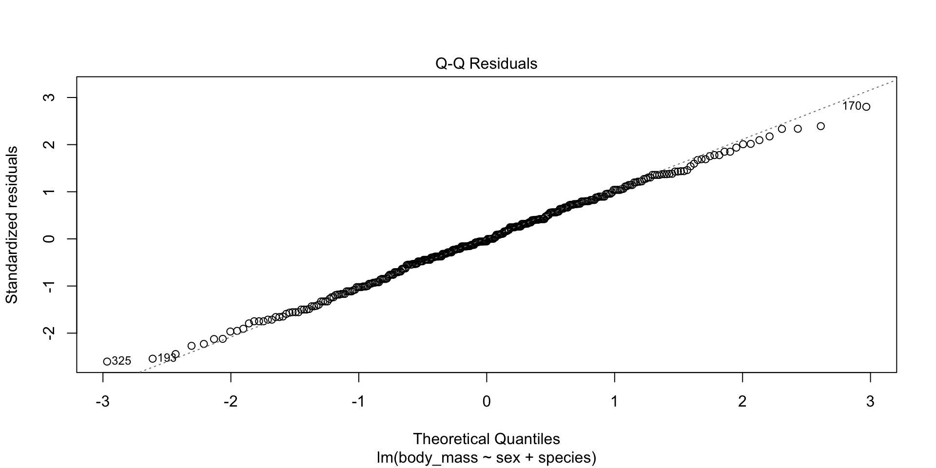
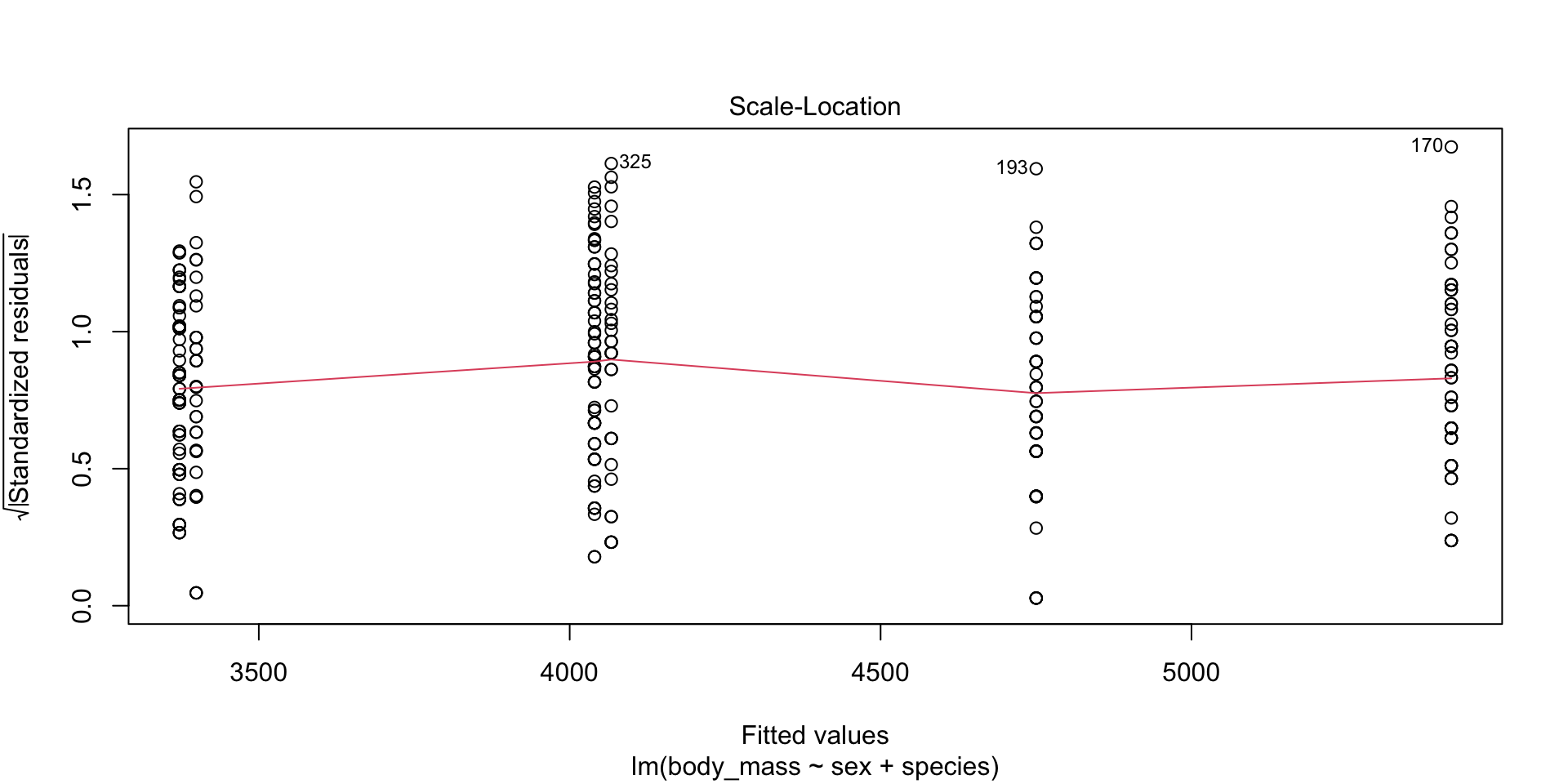
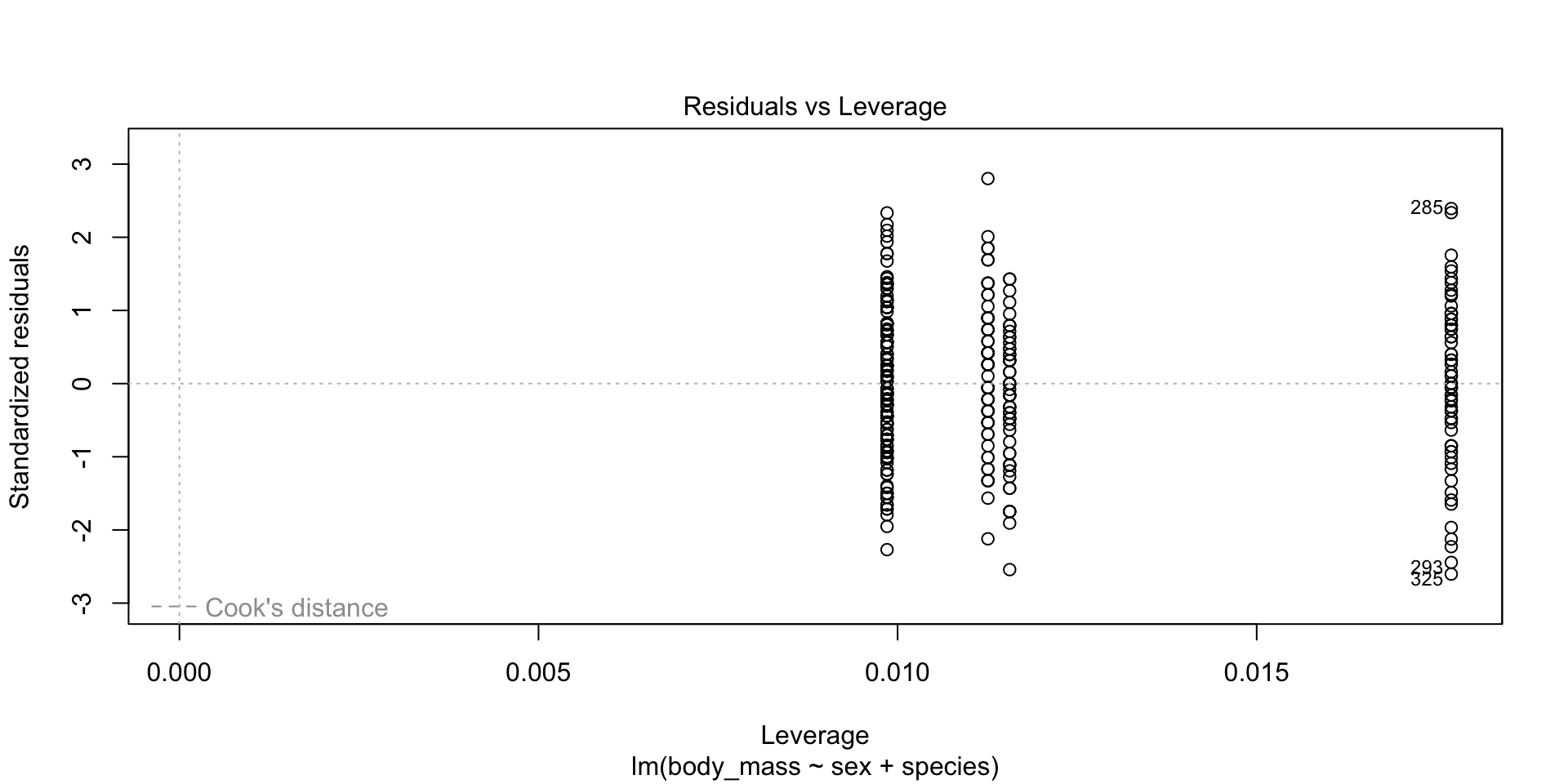
Model fit

You can plot the output of lm()

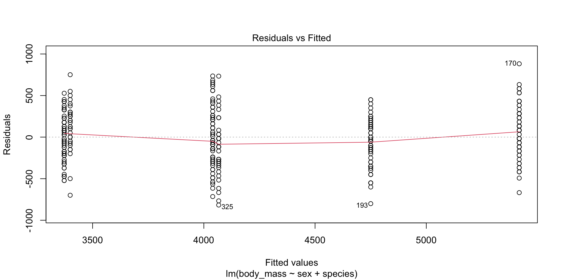
plot(regression_results)

Model summary

regression_results


Call:
lm(formula = body_mass ~ sex + species, data = data)

Coefficients:
     (Intercept)           sexmale  speciesChinstrap     speciesGentoo  
         3372.39            667.56             26.92           1377.86

summary(regression_results)


Call:
lm(formula = body_mass ~ sex + species, data = data)

Residuals:
    Min      1Q  Median      3Q     Max 
-816.87 -217.80  -16.87  227.61  882.20 

Coefficients:
                 Estimate Std. Error t value Pr(>|t|)    
(Intercept)       3372.39      31.43 107.308   <2e-16 ***
sexmale            667.56      34.70  19.236   <2e-16 ***
speciesChinstrap    26.92      46.48   0.579    0.563    
speciesGentoo     1377.86      39.10  35.236   <2e-16 ***
---
Signif. codes:  0 '***' 0.001 '**' 0.01 '*' 0.05 '.' 0.1 ' ' 1

Residual standard error: 316.6 on 329 degrees of freedom
  (11 observations deleted due to missingness)
Multiple R-squared:  0.8468,    Adjusted R-squared:  0.8454 
F-statistic: 606.1 on 3 and 329 DF,  p-value: < 2.2e-16

Accessing model results

names(regression_results)

 [1] "coefficients"  "residuals"     "effects"       "rank"         
 [5] "fitted.values" "assign"        "qr"            "df.residual"  
 [9] "na.action"     "contrasts"     "xlevels"       "call"         
[13] "terms"         "model"

Coefficients
Residuals
Terms

regression_results$coefficients

     (Intercept)          sexmale speciesChinstrap    speciesGentoo 
      3372.38681        667.55515         26.92385       1377.85803

regression_results$residuals

           1            2            3            5            6            7 
-289.9419594  427.6131923 -122.3868077   77.6131923 -389.9419594  252.6131923 
           8           13           14           15           16           17 
 635.0580406 -172.3868077 -239.9419594  360.0580406  327.6131923   77.6131923 
          18           19           20           21           22           23 
 460.0580406  -47.3868077  160.0580406   27.6131923 -439.9419594  427.6131923 
          24           25           26           27           28           29 
 -89.9419594 -239.9419594  427.6131923 -489.9419594 -172.3868077 -222.3868077 
          30           31           32           33           34           35 
 -89.9419594 -122.3868077 -139.9419594  -72.3868077 -139.9419594  -47.3868077 
          36           37           38           39           40           41 
 110.0580406  -89.9419594  177.6131923  -72.3868077  610.0580406 -222.3868077 
          42           43           44           45           46           47 
-139.9419594 -272.3868077  360.0580406 -372.3868077  560.0580406 -614.9419594 
          49           50           51           52           53           54 
  77.6131923  110.0580406  127.6131923  260.0580406   77.6131923   10.0580406 
          55           56           57           58           59           60 
-472.3868077 -339.9419594  177.6131923 -239.9419594 -522.3868077 -289.9419594 
          61           62           63           64           65           66 
-222.3868077  360.0580406  227.6131923   10.0580406 -522.3868077  -89.9419594 
          67           68           69           70           71           72 
 -22.3868077   60.0580406 -322.3868077  410.0580406  227.6131923 -139.9419594 
          73           74           75           76           77           78 
 177.6131923  110.0580406  327.6131923  210.0580406  327.6131923 -139.9419594 
          79           80           81           82           83           84 
 177.6131923  -39.9419594 -172.3868077  660.0580406  427.6131923  160.0580406 
          85           86           87           88           89           90 
 -22.3868077 -489.9419594 -239.9419594  127.6131923  -89.9419594  227.6131923 
          91           92           93           94           95           96 
 177.6131923  260.0580406   27.6131923  410.0580406  -72.3868077  260.0580406 
          97           98           99          100          101          102 
 327.6131923  310.0580406 -472.3868077   60.0580406  352.6131923  685.0580406 
         103          104          105          106          107          108 
-297.3868077  210.0580406 -447.3868077 -489.9419594  377.6131923 -139.9419594 
         109          110          111          112          113          114 
-197.3868077  735.0580406  452.6131923  560.0580406 -172.3868077  235.0580406 
         115          116          117          118          119          120 
 527.6131923   35.0580406 -472.3868077 -264.9419594  -22.3868077 -714.9419594 
         121          122          123          124          125          126 
-222.3868077 -539.9419594   77.6131923 -164.9419594 -322.3868077  -39.9419594 
         127          128          129          130          131          132 
 -97.3868077  260.0580406 -322.3868077  -39.9419594  -47.3868077 -539.9419594 
         133          134          135          136          137          138 
 127.6131923  435.0580406   52.6131923 -139.9419594 -197.3868077  -64.9419594 
         139          140          141          142          143          144 
  27.6131923  210.0580406   27.6131923 -564.9419594 -322.3868077 -314.9419594 
         145          146          147          148          149          150 
-372.3868077 -389.9419594  210.0580406  102.6131923   77.6131923 -289.9419594 
         151          152          153          154          155          156 
 327.6131923  -39.9419594 -250.2448382  282.2000101 -300.2448382  282.2000101 
         157          158          159          160          161          162 
 -17.7999899 -200.2448382   49.7551618 -217.7999899 -350.2448382 -267.7999899 
         163          164          165          166          167          168 
-100.2448382  132.2000101 -100.2448382  432.2000101 -550.2448382  432.2000101 
         169          170          171          172          173          174 
-600.2448382  882.2000101   49.7551618  -67.7999899  282.2000101  249.7551618 
         175          176          177          178          180          181 
-350.2448382 -367.7999899  249.7551618 -317.7999899  232.2000101 -150.2448382 
         182          183          184          185          186          187 
 132.2000101 -167.7999899  -50.2448382  299.7551618  632.2000101  399.7551618 
         188          189          190          191          192          193 
 -17.7999899  199.7551618 -167.7999899 -400.2448382  -67.7999899 -800.2448382 
         194          195          196          197          198          199 
 282.2000101 -450.2448382 -667.7999899  132.2000101  149.7551618 -550.2448382 
         200          201          202          203          204          205 
 -17.7999899  349.7551618 -117.7999899   99.7551618 -117.7999899 -350.2448382 
         206          207          208          209          210          211 
-417.7999899  149.7551618 -367.7999899 -450.2448382 -417.7999899 -300.2448382 
         212          213          214          215          216          217 
 132.2000101 -550.2448382 -117.7999899 -350.2448382  232.2000101  -50.2448382 
         218          220          221          222          223          224 
 282.2000101  382.2000101  -50.2448382  132.2000101   -0.2448382 -417.7999899 
         225          226          227          228          229          230 
-317.7999899  449.7551618  -50.2448382  382.2000101 -150.2448382  582.2000101 
         231          232          233          234          235          236 
  -0.2448382  532.2000101 -125.2448382   32.2000101  -25.2448382  -67.7999899 
         237          238          239          240          241          242 
  -0.2448382  182.2000101 -150.2448382 -117.7999899  124.7551618  132.2000101 
         243          244          245          246          247          248 
 199.7551618  -17.7999899   -0.2448382  232.2000101   99.7551618 -217.7999899 
         249          250          251          252          253          254 
-492.7999899  124.7551618 -125.2448382 -167.7999899   99.7551618  182.2000101 
         255          256          258          259          260          261 
 224.7551618   82.2000101   82.2000101  -50.2448382   82.2000101 -175.2448382 
         262          263          264          265          266          267 
  82.2000101  249.7551618  532.2000101 -100.2448382   82.2000101 -375.2448382 
         268          270          271          273          274          275 
 432.2000101  582.2000101  174.7551618   99.7551618  332.2000101  449.7551618 
         276          277          278          279          280          281 
 -17.7999899  100.6893406 -166.8658111 -416.8658111  125.6893406 -341.8658111 
         282          283          284          285          286          287 
 550.6893406 -149.3106594 -316.8658111  750.6893406 -366.8658111  400.6893406 
         288          289          290          291          292          293 
-291.8658111  300.6893406  -16.8658111  175.6893406  -16.8658111 -766.8658111 
         294          295          296          297          298          299 
 300.6893406   50.6893406  333.1341889  200.6893406 -666.8658111 -499.3106594 
         300          301          302          303          304          305 
-266.8658111  -99.3106594   83.1341889    0.6893406 -266.8658111  300.6893406 
         306          307          308          309          310          311 
 483.1341889 -199.3106594  233.1341889  -49.3106594   33.1341889 -466.8658111 
         312          313          314          315          316          317 
 500.6893406  450.6893406  733.1341889 -699.3106594  433.1341889 -116.8658111 
         318          319          320          321          322          323 
 250.6893406 -516.8658111  100.6893406  275.6893406  383.1341889    0.6893406 
         324          325          326          327          328          329 
 233.1341889 -816.8658111  275.6893406  -74.3106594 -116.8658111  200.6893406 
         330          331          332          333          334          335 
 -16.8658111  -49.3106594 -616.8658111 -149.3106594  -16.8658111 -266.8658111 
         336          337          338          339          340          341 
 125.6893406 -116.8658111  250.6893406  250.6893406  -66.8658111    0.6893406 
         342          343          344 
-291.8658111   33.1341889  375.6893406

regression_results$terms

body_mass ~ sex + species
attr(,"variables")
list(body_mass, sex, species)
attr(,"factors")
          sex species
body_mass   0       0
sex         1       0
species     0       1
attr(,"term.labels")
[1] "sex"     "species"
attr(,"order")
[1] 1 1
attr(,"intercept")
[1] 1
attr(,"response")
[1] 1
attr(,".Environment")
<environment: R_GlobalEnv>
attr(,"predvars")
list(body_mass, sex, species)
attr(,"dataClasses")
  body_mass         sex     species 
  "numeric" "character" "character"

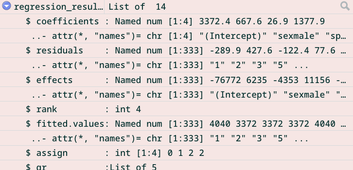
Accessing model results

gtsummary has a function for this ¹

tbl_regression(
  regression_results,
  intercept = TRUE,
  pvalue_fun = label_style_pvalue(digits = 3)
  )

Characteristic	Beta	95% CI	p-value
(Intercept)	3,372	3,311, 3,434	<0.001
sex
female	—	—
male	668	599, 736	<0.001
species
Adelie	—	—
Chinstrap	27	-65, 118	0.563
Gentoo	1,378	1,301, 1,455	<0.001
Abbreviation: CI = Confidence Interval

Available models*

Base R:

Linear lm()
Generalised linear glm()
Time series ar(), arima(), arima0()

Packages for common models:

survival for survival analysis
gee for generalised estimating equations
lme4 and glmmTMB for mixed-effects models
brms Bayesian stuff
gam and gamlss for generalised additive models

Questions!

Data wrangling

Reading in data

Which package to use?

readr for reading .csv files
readxl for Excel files (.xls and .xlsx)
haven for Stata, SPSS, and SAS files
googlesheets4 for reading directly from Google Sheets

Tip

See the reading data cheatsheet: https://github.com/rstudio/cheatsheets/blob/main/data-import.pdf

Reading in data

If the data are clean, it’s not complicated

messy_data <- read_csv("data/penguins.csv")

# Function arguments
read_csv(
  file,
  col_names = TRUE,
  col_types = NULL,
  col_select = NULL,
  id = NULL,
  locale = default_locale(),
  na = c("", "NA"),
  quoted_na = deprecated(),
  quote = "\"",
  comment = "",
  trim_ws = TRUE,
  skip = 0,
  n_max = Inf,
  guess_max = min(1000, n_max),
  name_repair = "unique",
  num_threads = readr_threads(),
  progress = show_progress(),
  show_col_types = should_show_types(),
  skip_empty_rows = TRUE,
  lazy = should_read_lazy()
)

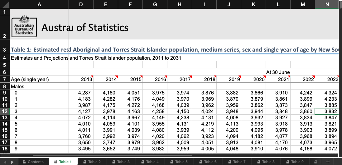
Reading in messy data

Data aren’t always machine-readable, especially from the ABS

First sheet
Actual data

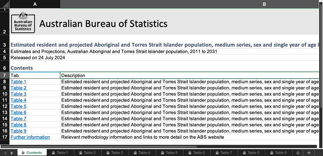
Reading in messy data

library(readxl)

messy_data <- read_excel(
  "data/32380DO004_20112031.xlsx",
  
  
)

library(readxl)

messy_data <- read_excel(
  "data/32380DO004_20112031.xlsx",
  sheet = "Table 1",
  
)

library(readxl)

messy_data <- read_excel(
  "data/32380DO004_20112031.xlsx",
  sheet = "Table 1",
  skip = 6
)

# Function arguments
read_excel(
  path,
  sheet = NULL,
  range = NULL,
  col_names = TRUE,
  col_types = NULL,
  na = "",
  trim_ws = TRUE,
  skip = 0,
  n_max = Inf,
  guess_max = min(1000, n_max),
  progress = readxl_progress(),
  .name_repair = "unique"
)

Viewing data

Look at your data!

View() or click on the object
type the name in the console (data)
use head() to see a snapshot
use dplyr::glimpse()

View
print
head
glimpse

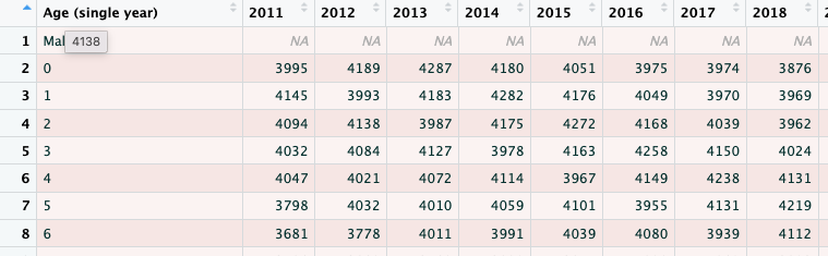
messy_data

# A tibble: 136 × 22
   `Age (single year)` `2011` `2012` `2013` `2014` `2015` `2016` `2017` `2018`
   <chr>                <dbl>  <dbl>  <dbl>  <dbl>  <dbl>  <dbl>  <dbl>  <dbl>
 1 Males                   NA     NA     NA     NA     NA     NA     NA     NA
 2 0                     3995   4189   4287   4180   4051   3975   3974   3876
 3 1                     4145   3993   4183   4282   4176   4049   3970   3969
 4 2                     4094   4138   3987   4175   4272   4168   4039   3962
 5 3                     4032   4084   4127   3978   4163   4258   4150   4024
 6 4                     4047   4021   4072   4114   3967   4149   4238   4131
 7 5                     3798   4032   4010   4059   4101   3955   4131   4219
 8 6                     3681   3778   4011   3991   4039   4080   3939   4112
 9 7                     3506   3662   3760   3992   3974   4020   4062   3923
10 8                     3275   3493   3650   3747   3979   3962   4009   4051
# ℹ 126 more rows
# ℹ 13 more variables: `2019` <dbl>, `2020` <dbl>, `2021` <dbl>, `2022` <dbl>,
#   `2023` <dbl>, `2024` <dbl>, `2025` <dbl>, `2026` <dbl>, `2027` <dbl>,
#   `2028` <dbl>, `2029` <dbl>, `2030` <dbl>, `2031` <dbl>

head(messy_data)

# A tibble: 6 × 22
  `Age (single year)` `2011` `2012` `2013` `2014` `2015` `2016` `2017` `2018`
  <chr>                <dbl>  <dbl>  <dbl>  <dbl>  <dbl>  <dbl>  <dbl>  <dbl>
1 Males                   NA     NA     NA     NA     NA     NA     NA     NA
2 0                     3995   4189   4287   4180   4051   3975   3974   3876
3 1                     4145   3993   4183   4282   4176   4049   3970   3969
4 2                     4094   4138   3987   4175   4272   4168   4039   3962
5 3                     4032   4084   4127   3978   4163   4258   4150   4024
6 4                     4047   4021   4072   4114   3967   4149   4238   4131
# ℹ 13 more variables: `2019` <dbl>, `2020` <dbl>, `2021` <dbl>, `2022` <dbl>,
#   `2023` <dbl>, `2024` <dbl>, `2025` <dbl>, `2026` <dbl>, `2027` <dbl>,
#   `2028` <dbl>, `2029` <dbl>, `2030` <dbl>, `2031` <dbl>

glimpse(messy_data)

Rows: 136
Columns: 22
$ `Age (single year)` <chr> "Males", "0", "1", "2", "3", "4", "5", "6", "7", "…
$ `2011`              <dbl> NA, 3995, 4145, 4094, 4032, 4047, 3798, 3681, 3506…
$ `2012`              <dbl> NA, 4189, 3993, 4138, 4084, 4021, 4032, 3778, 3662…
$ `2013`              <dbl> NA, 4287, 4183, 3987, 4127, 4072, 4010, 4011, 3760…
$ `2014`              <dbl> NA, 4180, 4282, 4175, 3978, 4114, 4059, 3991, 3992…
$ `2015`              <dbl> NA, 4051, 4176, 4272, 4163, 3967, 4101, 4039, 3974…
$ `2016`              <dbl> NA, 3975, 4049, 4168, 4258, 4149, 3955, 4080, 4020…
$ `2017`              <dbl> NA, 3974, 3970, 4039, 4150, 4238, 4131, 3939, 4062…
$ `2018`              <dbl> NA, 3876, 3969, 3962, 4024, 4131, 4219, 4112, 3923…
$ `2019`              <dbl> NA, 3882, 3870, 3959, 3948, 4008, 4113, 4200, 4094…
$ `2020`              <dbl> NA, 3866, 3879, 3862, 3944, 3932, 3993, 4095, 4182…
$ `2021`              <dbl> NA, 3910, 3861, 3873, 3848, 3927, 3918, 3978, 4077…
$ `2022`              <dbl> NA, 4242, 3899, 3847, 3860, 3834, 3913, 3903, 3968…
$ `2023`              <dbl> NA, 4324, 4233, 3885, 3832, 3847, 3821, 3899, 3894…
$ `2024`              <dbl> NA, 4394, 4315, 4219, 3870, 3818, 3833, 3808, 3890…
$ `2025`              <dbl> NA, 4467, 4385, 4301, 4204, 3856, 3803, 3820, 3801…
$ `2026`              <dbl> NA, 4540, 4458, 4372, 4286, 4189, 3841, 3789, 3813…
$ `2027`              <dbl> NA, 4613, 4531, 4444, 4357, 4271, 4176, 3826, 3780…
$ `2028`              <dbl> NA, 4691, 4605, 4517, 4428, 4343, 4257, 4162, 3818…
$ `2029`              <dbl> NA, 4756, 4682, 4590, 4501, 4413, 4329, 4242, 4153…
$ `2030`              <dbl> NA, 4821, 4747, 4667, 4574, 4486, 4398, 4314, 4233…
$ `2031`              <dbl> NA, 4876, 4812, 4732, 4650, 4559, 4471, 4382, 4305…

Renaming

janitor::clean_names() is a starting point

dplyr::rename() and dplyr::rename_with() let you specify names

Current names
clean_names
rename
rename_with
Example

names(messy_data)

 [1] "Age (single year)" "2011"              "2012"             
 [4] "2013"              "2014"              "2015"             
 [7] "2016"              "2017"              "2018"             
[10] "2019"              "2020"              "2021"             
[13] "2022"              "2023"              "2024"             
[16] "2025"              "2026"              "2027"             
[19] "2028"              "2029"              "2030"             
[22] "2031"

messy_data |> 
  clean_names() |> 
  names()

 [1] "age_single_year" "x2011"           "x2012"           "x2013"          
 [5] "x2014"           "x2015"           "x2016"           "x2017"          
 [9] "x2018"           "x2019"           "x2020"           "x2021"          
[13] "x2022"           "x2023"           "x2024"           "x2025"          
[17] "x2026"           "x2027"           "x2028"           "x2029"          
[21] "x2030"           "x2031"

messy_data |> 
  rename(
    age = `Age (single year)`
  ) |> 
  names()

 [1] "age"  "2011" "2012" "2013" "2014" "2015" "2016" "2017" "2018" "2019"
[11] "2020" "2021" "2022" "2023" "2024" "2025" "2026" "2027" "2028" "2029"
[21] "2030" "2031"

messy_data |> 
  rename_with(
    \(x)
    paste0("y", x),
    `2011`:`2031`
  ) |> 
  names()

 [1] "Age (single year)" "y2011"             "y2012"            
 [4] "y2013"             "y2014"             "y2015"            
 [7] "y2016"             "y2017"             "y2018"            
[10] "y2019"             "y2020"             "y2021"            
[13] "y2022"             "y2023"             "y2024"            
[16] "y2025"             "y2026"             "y2027"            
[19] "y2028"             "y2029"             "y2030"            
[22] "y2031"

messy_data <- messy_data |> 
  clean_names() |> 
  rename(
    age = age_single_year
  )
names(messy_data)

 [1] "age"   "x2011" "x2012" "x2013" "x2014" "x2015" "x2016" "x2017" "x2018"
[10] "x2019" "x2020" "x2021" "x2022" "x2023" "x2024" "x2025" "x2026" "x2027"
[19] "x2028" "x2029" "x2030" "x2031"

Selecting

Keep or remove columns using select()

Keep
Drop
Ranges
Selectors
Example

messy_data |> 
  select(age, x2011) |> 
  names()

[1] "age"   "x2011"

Separate names using commas ,

messy_data |> 
  select(-age) |> 
  names()

 [1] "x2011" "x2012" "x2013" "x2014" "x2015" "x2016" "x2017" "x2018" "x2019"
[10] "x2020" "x2021" "x2022" "x2023" "x2024" "x2025" "x2026" "x2027" "x2028"
[19] "x2029" "x2030" "x2031"

Use a minus - to drop a variable

messy_data |> 
  select(age, x2011:x2016) |> 
  names()

[1] "age"   "x2011" "x2012" "x2013" "x2014" "x2015" "x2016"

Use a colon : connecting two variables to select them and everything in between

messy_data |> 
  select(
    contains("202"),
    starts_with("x"),
    where(is.numeric)
  ) |> 
  names()

 [1] "x2020" "x2021" "x2022" "x2023" "x2024" "x2025" "x2026" "x2027" "x2028"
[10] "x2029" "x2011" "x2012" "x2013" "x2014" "x2015" "x2016" "x2017" "x2018"
[19] "x2019" "x2030" "x2031"

contains matches against a pattern
starts_with only looks at the start
where keeps columns that meet a criteria
See the tidyselect package

messy_data <- messy_data |> 
  select(
    age,
    contains("202")
  )

messy_data

# A tibble: 136 × 11
   age   x2020 x2021 x2022 x2023 x2024 x2025 x2026 x2027 x2028 x2029
   <chr> <dbl> <dbl> <dbl> <dbl> <dbl> <dbl> <dbl> <dbl> <dbl> <dbl>
 1 Males    NA    NA    NA    NA    NA    NA    NA    NA    NA    NA
 2 0      3866  3910  4242  4324  4394  4467  4540  4613  4691  4756
 3 1      3879  3861  3899  4233  4315  4385  4458  4531  4605  4682
 4 2      3862  3873  3847  3885  4219  4301  4372  4444  4517  4590
 5 3      3944  3848  3860  3832  3870  4204  4286  4357  4428  4501
 6 4      3932  3927  3834  3847  3818  3856  4189  4271  4343  4413
 7 5      3993  3918  3913  3821  3833  3803  3841  4176  4257  4329
 8 6      4095  3978  3903  3899  3808  3820  3789  3826  4162  4242
 9 7      4182  4077  3968  3894  3890  3801  3813  3780  3818  4153
10 8      4081  4170  4073  3965  3893  3888  3799  3811  3778  3815
# ℹ 126 more rows

We’ve kept the age variable and counts for the 2020s

Filtering

Keep or remove rows using dplyr::filter()

One
Two
OR
%in%
Example

messy_data |> 
  filter(age == "18") |> 
  nrow()

[1] 2

age is a character
== is how to specify an equality

messy_data |> 
  filter(
    age == "18",
    x2020 > 1000
    ) |> 
  nrow()

[1] 2

messy_data |> 
  filter(
    age == "18" &
      x2020 > 1000
    ) |> 
  nrow()

[1] 2

x2011 is a number
Separating conditions with a comma is the same as using &

messy_data |> 
  filter(
    age == "18" |
      age == "19"
    ) |> 
  nrow()

[1] 4

The vertical bar | is how to specify OR
If either condition is true, the row is kept

messy_data |> 
  filter(
    age %in% c("18","19","20")
    ) |> 
  nrow()

[1] 6

messy_data <- messy_data |> 
  filter(
    between(as.numeric(age), 18, 40) | 
      age %in% c("Males", "Females")
    ) 

messy_data

# A tibble: 48 × 11
   age   x2020 x2021 x2022 x2023 x2024 x2025 x2026 x2027 x2028 x2029
   <chr> <dbl> <dbl> <dbl> <dbl> <dbl> <dbl> <dbl> <dbl> <dbl> <dbl>
 1 Males    NA    NA    NA    NA    NA    NA    NA    NA    NA    NA
 2 18     3355  3259  3449  3606  3694  3921  3911  3944  3978  3856
 3 19     3245  3336  3237  3423  3580  3669  3894  3887  3919  3952
 4 20     3147  3222  3309  3213  3395  3552  3643  3867  3861  3893
 5 21     3061  3123  3196  3281  3187  3366  3524  3614  3837  3834
 6 22     3000  3037  3105  3178  3261  3171  3347  3505  3596  3817
 7 23     2926  2984  3017  3084  3156  3237  3152  3325  3482  3573
 8 24     2819  2905  2965  2996  3063  3134  3214  3132  3302  3458
 9 25     2877  2800  2877  2938  2970  3035  3106  3185  3105  3273
10 26     2590  2850  2773  2848  2911  2943  3008  3079  3156  3079
# ℹ 38 more rows

We’ve kept only ages 18 to 40, or where age is Males or Females

Modifying

Update an existing column or make a new one using mutate()

One variable
Multiple variables
if_else
case_when
Example

messy_data |> 
  mutate(
    var_1 = "1"
  )

Single equals = to specify what the variable (var_1) should be

messy_data |> 
  mutate(
    var_1 = "1",
    var_2 = 2,
    var_3 = as.numeric(var_1) + var_2
  )

Separate variables using commas
Creating a variable on an earlier line means you can refer to it within the same mutate()

messy_data |> 
  mutate(
    var_1 = if_else(
      condition = age %in% c("18", "19", "20"),
      true = 1,
      false = 0,
      missing = 0
    )
  )

missing specifies what to do if the value is NA

messy_data |> 
  mutate(
    age = as.numeric(age),
    var_1 = case_when(
      age %in% c(18, 19, 20) ~ "18 to 20",
      between(age, 21, 30) ~ "21 to 30",
      between(age, 30, 40) ~ "30 to 40",
      .default = "Other"
    )
  )

the condition (left-side) must evaluate to TRUE or FALSE
the value to assign if this condition is true (right-side)
separated by a tilde ~
the .default is NA if you don’t specify anything
applies conditions from top to bottom

messy_data <- messy_data |> 
  mutate(
    sex = case_when(
      age == "Males" ~ age,
      age == "Females" ~ age,
      .default = NA
    ),
    age = as.numeric(age),
    age_group = case_when(
      between(age, 18, 24) ~ "18 to 24",
      between(age, 25, 40) ~ "25 to 40"
    )
  )

sex is extracted from the age variable
age is numeric now
age_group is based on age ranges

Filling in missing data

dplyr::fill() fills in missing data using the last non-missing values

Before
After

messy_data$sex

 [1] "Males"   NA        NA        NA        NA        NA        NA       
 [8] NA        NA        NA        NA        NA        NA        NA       
[15] NA        NA        NA        NA        NA        NA        NA       
[22] NA        NA        NA        "Females" NA        NA        NA       
[29] NA        NA        NA        NA        NA        NA        NA       
[36] NA        NA        NA        NA        NA        NA        NA       
[43] NA        NA        NA        NA        NA        NA

# Function arguments
fill(
  messy_data, 
  ..., 
  .by = NULL, 
  .direction = c("down", "up", "downup", "updown")
)

messy_data <- messy_data |> 
  fill(sex, .direction = "down")

messy_data$sex

 [1] "Males"   "Males"   "Males"   "Males"   "Males"   "Males"   "Males"  
 [8] "Males"   "Males"   "Males"   "Males"   "Males"   "Males"   "Males"  
[15] "Males"   "Males"   "Males"   "Males"   "Males"   "Males"   "Males"  
[22] "Males"   "Males"   "Males"   "Females" "Females" "Females" "Females"
[29] "Females" "Females" "Females" "Females" "Females" "Females" "Females"
[36] "Females" "Females" "Females" "Females" "Females" "Females" "Females"
[43] "Females" "Females" "Females" "Females" "Females" "Females"

# Function arguments
fill(
  messy_data, 
  ..., 
  .by = NULL, 
  .direction = c("down", "up", "downup", "updown")
)

Reshaping data

Use pivot_longer() and pivot_wider() to reshape datasets

Longer
Wider

messy_data <- messy_data |> 
  filter(!is.na(age)) |> 
  pivot_longer(
    cols = starts_with("x"),
    names_to = "year",
    values_to = "count",
  )

messy_data

# A tibble: 460 × 5
     age sex   age_group year  count
   <dbl> <chr> <chr>     <chr> <dbl>
 1    18 Males 18 to 24  x2020  3355
 2    18 Males 18 to 24  x2021  3259
 3    18 Males 18 to 24  x2022  3449
 4    18 Males 18 to 24  x2023  3606
 5    18 Males 18 to 24  x2024  3694
 6    18 Males 18 to 24  x2025  3921
 7    18 Males 18 to 24  x2026  3911
 8    18 Males 18 to 24  x2027  3944
 9    18 Males 18 to 24  x2028  3978
10    18 Males 18 to 24  x2029  3856
# ℹ 450 more rows

messy_data <- messy_data |> 
  filter(!is.na(age)) |> 
  pivot_wider(
    names_from = sex,
    values_from = count,
  )

messy_data

# A tibble: 230 × 5
     age age_group year  Males Females
   <dbl> <chr>     <chr> <dbl>   <dbl>
 1    18 18 to 24  x2020  3355    3089
 2    18 18 to 24  x2021  3259    3110
 3    18 18 to 24  x2022  3449    3182
 4    18 18 to 24  x2023  3606    3326
 5    18 18 to 24  x2024  3694    3551
 6    18 18 to 24  x2025  3921    3798
 7    18 18 to 24  x2026  3911    3747
 8    18 18 to 24  x2027  3944    3770
 9    18 18 to 24  x2028  3978    3778
10    18 18 to 24  x2029  3856    3709
# ℹ 220 more rows

Grouping

Use group_by() or the .by = argument

group_by()
.by =

messy_data |> 
  group_by(age_group) |> 
  summarise(
    n_total = sum(Males) + sum(Females)
  ) |> 
  ungroup()

# A tibble: 2 × 2
  age_group n_total
  <chr>       <dbl>
1 18 to 24   464094
2 25 to 40   772088

When you use group_by(), the output remains grouped.
Use ungroup() to remove the grouping

messy_data |> 
  summarise(
    n_total = sum(Males) + sum(Females),
    .by = age_group
  )

# A tibble: 2 × 2
  age_group n_total
  <chr>       <dbl>
1 18 to 24   464094
2 25 to 40   772088

.by applies the grouping just for that operation, so grouping doesn’t persist
Available for:
- filter() and filter_out()
- mutate()
- summarise()
- slice() functions

Let’s practice!

Going back to the penguins dataset

Drop the flip_len variable

data |> 
  select(-flipper_len)

Rename bill_len to bill_length and bill_dep to bill_depth

data |> 
  rename(
    bill_length = bill_len,
    bill_depth = bill_dep
  )

Create a variable for the ratio of bill length to bill depth

data |> 
  mutate(
    bill_length_depth_ratio = bill_length / bill_depth
  )

Reshape the two bill variables into a longer format

data |> 
  pivot_longer(
    contains("bill"),
    names_to = "bill_measure",
    values_to = "bill_value"
  )

Question time

Where to next?

R resources:

R for Data Science https://r4ds.hadley.nz/
Advanced R https://adv-r.hadley.nz/index.html
The Epidemiologist R Handbook https://epirhandbook.com/en/
- A little out of date, but still relevant

Consider learning Quarto (https://quarto.org/), for reproducible workflows

Feedback?

I don’t want it!

(just kidding)

Chat to me now

Email me: benjamin.harrap@anu.edu.au

Getting to know R and RStudio

Hello

Hello

Outline

What you’ll come away with

Housekeeping

Important context

R vs. RStudio

RStudio

RStudio

RStudio

RStudio

.RProj files

Working directory

Absolute vs. relative locations

Absolute vs. relative locations

Packages

The tidyverse

Package conflicts

Question time

Let’s practice!

Coding in R

penguins

Comments

Elements of code

Assignment (<-)

Accessing elements of an object

Pipes (|>)

Keyboard shortcuts

Common types of things

Missing

Human-readable code

Common errors

Error messages

Help files

Let’s practice!

Question time

Break time!

Example workflow

Example workflow

Summaries and tables

dplyr::summarise()

janitor::tabyl()

janitor::tabyl()

gtsummary

tbl_summary()

tbl_summary()

tbl_summary()

tbl_summary()

tbl_summary()

Other packages for tables

Let’s practice!

Data visualisation

Package options

ggplot2

ggplot2

Scatter plot

Bar plot

Bar plot

Line graph

Line graph

Questions?

Customising a plot

Customising axes

Customising the legend

Customising with a theme

Adding an element

Adding a facet

Saving the output

Let’s practice!

Questions?

Regression

Model notation

Model fit

Model summary

Accessing model results

Accessing model results

Available models*

Questions!

Data wrangling

`.RProj` files

The `tidyverse`

`penguins`

Assignment (`<-`)

Pipes (`|>`)

`dplyr::summarise()`

`janitor::tabyl()`

`janitor::tabyl()`

`gtsummary`

`tbl_summary()`

`tbl_summary()`

`tbl_summary()`

`tbl_summary()`

`tbl_summary()`

`ggplot2`

`ggplot2`