Coding

(in Stata and R)

Ben Harrap

2025-02-14

Overview

In this session we’ll cover:

R fundamentals
Common coding tasks
- Concept
- Data
- Code (Stata and R)

R fundamentals

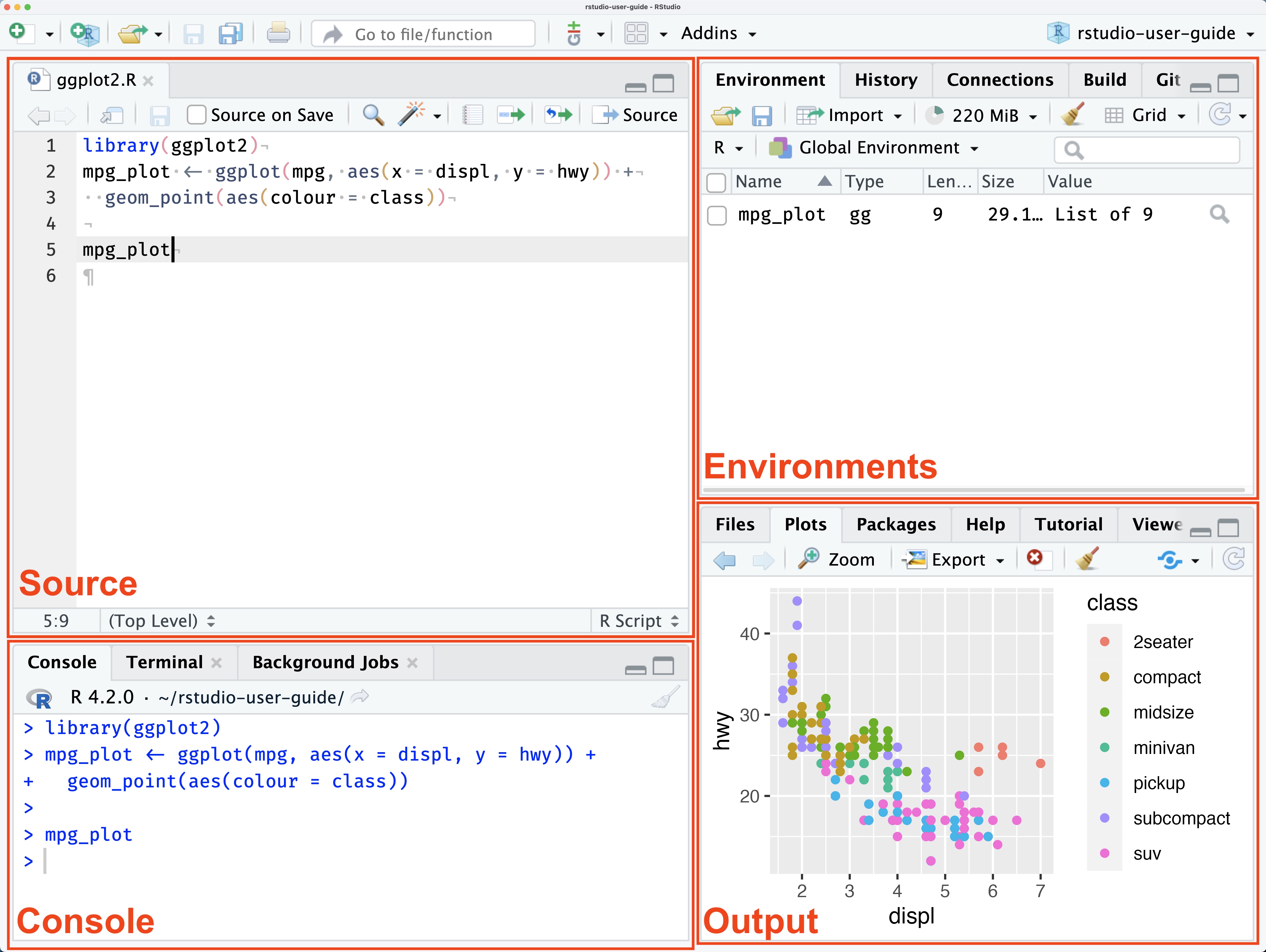
R and RStudio

R is the language that the code is written in.

RStudio is the IDE many people use to write R code in.

At a minimum you need to install R (r-project.org)

IDE options include:

RStudio (posit.co/products/open-source/rstudio)
Positron (positron.posit.co)
VS Code (code.visualstudio.com)

A screenshot of the RStudio IDE. Source: Posit

Packages

One of the greatest strengths of R is that it is open-source and there are an enormous number of packages available.

A package is a collection of functions usually written around a particular goal or task.

Packages I recommend:

tidyverse which includes:
- dplyr for data manipulation
- ggplot2 for data visualisation
- stringr for working with text data
- lubridate for working with dates
janitor which has many useful cleaning tools
haven for reading Stata files

Packages

First you need to install packages:

install.packages("tidyverse")

Then you need to load them into your session using library():

library(tidyverse) # Imports lots of useful packages
library(haven) # For reading Stata files (and SPSS and more)
library(janitor) # Handy cleaning functions
library(gt) # For nice tables

Assignment

In Stata, you load one dataset and all commands are executed in relation to the currently loaded dataset.

In R, the default is for commands to output their result in the console.

This means you need to assign the output of your commands to something if you want to store it.

Assignment

If we read in a dataset without assigning anything, it just gets displayed:

read_dta("data/auto.dta")

# A tibble: 74 × 12
   make        price   mpg rep78 headroom trunk weight length  turn displacement
   <chr>       <dbl> <dbl> <dbl>    <dbl> <dbl>  <dbl>  <dbl> <dbl>        <dbl>
 1 AMC Concord  4099    22     3      2.5    11   2930    186    40          121
 2 AMC Pacer    4749    17     3      3      11   3350    173    40          258
 3 AMC Spirit   3799    22    NA      3      12   2640    168    35          121
 4 Buick Cent…  4816    20     3      4.5    16   3250    196    40          196
 5 Buick Elec…  7827    15     4      4      20   4080    222    43          350
 6 Buick LeSa…  5788    18     3      4      21   3670    218    43          231
 7 Buick Opel   4453    26    NA      3      10   2230    170    34          304
 8 Buick Regal  5189    20     3      2      16   3280    200    42          196
 9 Buick Rivi… 10372    16     3      3.5    17   3880    207    43          231
10 Buick Skyl…  4082    19     3      3.5    13   3400    200    42          231
# ℹ 64 more rows
# ℹ 2 more variables: gear_ratio <dbl>, foreign <dbl+lbl>

Instead we have to give it a name and assign to the environment:

data <- read_dta("data/auto.dta")

Multiple datasets

Being able to have many things assigned in the environment at once opens up many possibilities:

Working on multiple datasets simultaneously
- Easier than working with Stata’s frame
Creating subsets of data
- More powerful version of Stata’s preserve and restore
Outputs from multiple analyses are readily available
- Model results, data visualisations

Pipes

In Stata, you write lines of code that get executed one after the other, individually and sequentially.

sysuse auto
drop if foreign == 1
gen wgt_len_ratio = weight/length
gen brand = substr(make, 1, ustrpos(make, " ")-1)
sort brand
by brand: summarize wgt_len_ratio

In R, you can create pipelines using pipes (|>) to link functions together and avoid having to repeatedly refer to the data you want to work with.

Pipes

Without pipes

auto <- read_dta("/Applications/Stata/auto.dta")
auto <- filter(auto, foreign == 0)
auto <- mutate(auto,
               wgt_len_ratio = weight / length,
               brand = str_extract(make, "\\w+"))
summarise(auto,
          n = n(),
          mean = mean(wgt_len_ratio),
          sd = sd(wgt_len_ratio),
          .by = brand)

With pipes

auto <- read_dta("/Applications/Stata/auto.dta")
auto |>
  filter(foreign == 0) |>
  mutate(wgt_len_ratio = weight / length,
         brand = str_extract(make, "\\w+")) |>
  summarise(
    n = n(),
    mean = mean(wgt_len_ratio),
    sd = sd(wgt_len_ratio),
    .by = brand)

First step: Get the data

Reading in a data file

The data you want to work with is contained in a file located somewhere.

To start using the data you need to consider:

The location of the file
- Is the data on your computer? A shared drive? An online location?
- Are you using the absolute or relative pathway?
- How are others going to run your code?
The format of the file (.dta,.xlsx,.csv,.txt,.SAV)

A note on folder structure

Relative vs. absolute directories

Users/Ben/Documents/GitHub/workshops/2025-02-14-coding-in-stata-and-r/data/auto.dta
./data/auto.dta

Network locations, root location different according to machine type.

Generally speaking, avoid using absolute pathways when possible.

Navigate to other directories from the current working directory using .. to go ‘up’ a folder:

../2024-08-20-admin-data/img/aihw.PNG

A note on directories

In Stata you would set your working directory using cd, such as

cd "/Users/ben/Documents/GitHub/workshops/2025-02-14-coding-in-stata-and-r"

In R you can use setwd() to set your working directory

setwd("/Users/ben/Documents/GitHub/workshops/2025-02-14-coding-in-stata-and-r")

Alternatively, use R projects (.Rproj)

- 2025-02-14-coding-in-stata-and-r
  - _brand.yml
  - 2025-02-14-coding-in-stata-and-r.Rproj
  - slides.html
  - slides.qmd
  - data
  - img

For a file in the same location as the current working directory:

use auto

For a file that is in another folder:

use "data/auto.dta"

For a file that is online:

import delimited "https://raw.githubusercontent.com/allisonhorst/palmerpenguins/refs/heads/main/inst/extdata/penguins_raw.csv"

For a file in the same location as the current working directory:

data <- read_dta("auto.dta")

For a file that is in another folder:

data <- read_dta("data/auto.dta")

For a file that is online:

data <- read_csv("https://raw.githubusercontent.com/allisonhorst/palmerpenguins/refs/heads/main/inst/extdata/penguins_raw.csv")

Overview of the data

Raw data containing observations of three different types of penguins, made available through https://allisonhorst.github.io/palmerpenguins/

gt(data |> slice_sample(n = 10))

studyName	Sample Number	Species	Region	Island	Stage	Individual ID	Clutch Completion	Date Egg	Culmen Length (mm)	Culmen Depth (mm)	Flipper Length (mm)	Body Mass (g)	Sex	Delta 15 N (o/oo)	Delta 13 C (o/oo)	Comments
PAL0910	141	Adelie Penguin (Pygoscelis adeliae)	Anvers	Dream	Adult, 1 Egg Stage	N80A1	Yes	2009-11-14	40.2	17.1	193	3400	FEMALE	9.28810	-25.54976	NA
PAL0910	47	Chinstrap penguin (Pygoscelis antarctica)	Anvers	Dream	Adult, 1 Egg Stage	N87A1	Yes	2009-11-27	50.1	17.9	190	3400	FEMALE	9.46819	-24.45721	NA
PAL0809	54	Gentoo penguin (Pygoscelis papua)	Anvers	Biscoe	Adult, 1 Egg Stage	N14A2	Yes	2008-11-04	50.1	15.0	225	5000	MALE	8.50153	-26.61414	NA
PAL0910	65	Chinstrap penguin (Pygoscelis antarctica)	Anvers	Dream	Adult, 1 Egg Stage	N99A1	No	2009-11-21	43.5	18.1	202	3400	FEMALE	9.37608	-24.40753	Nest never observed with full clutch.
PAL0910	97	Gentoo penguin (Pygoscelis papua)	Anvers	Biscoe	Adult, 1 Egg Stage	N20A1	Yes	2009-11-18	49.4	15.8	216	4925	MALE	8.03624	-26.06594	NA
PAL0809	49	Gentoo penguin (Pygoscelis papua)	Anvers	Biscoe	Adult, 1 Egg Stage	N12A1	Yes	2008-11-02	44.9	13.3	213	5100	FEMALE	8.45167	-26.89644	NA
PAL0809	64	Adelie Penguin (Pygoscelis adeliae)	Anvers	Biscoe	Adult, 1 Egg Stage	N28A2	Yes	2008-11-13	41.1	18.2	192	4050	MALE	8.62264	-26.60023	NA
PAL0809	54	Adelie Penguin (Pygoscelis adeliae)	Anvers	Biscoe	Adult, 1 Egg Stage	N22A2	Yes	2008-11-09	42.0	19.5	200	4050	MALE	8.48095	-26.31460	NA
PAL0708	13	Gentoo penguin (Pygoscelis papua)	Anvers	Biscoe	Adult, 1 Egg Stage	N37A1	Yes	2007-11-29	45.5	13.7	214	4650	FEMALE	7.77672	-25.41680	NA
PAL0708	4	Chinstrap penguin (Pygoscelis antarctica)	Anvers	Dream	Adult, 1 Egg Stage	N62A2	Yes	2007-11-26	45.4	18.7	188	3525	FEMALE	8.64701	-24.62717	NA

Second step: Prepare the data

Renaming variables

Variables might be imported with difficult to work with names, so we want to rename them

head(data)

# A tibble: 6 × 17
  studyName `Sample Number` Species          Region Island Stage `Individual ID`
  <chr>               <dbl> <chr>            <chr>  <chr>  <chr> <chr>          
1 PAL0708                 1 Adelie Penguin … Anvers Torge… Adul… N1A1           
2 PAL0708                 2 Adelie Penguin … Anvers Torge… Adul… N1A2           
3 PAL0708                 3 Adelie Penguin … Anvers Torge… Adul… N2A1           
4 PAL0708                 4 Adelie Penguin … Anvers Torge… Adul… N2A2           
5 PAL0708                 5 Adelie Penguin … Anvers Torge… Adul… N3A1           
6 PAL0708                 6 Adelie Penguin … Anvers Torge… Adul… N3A2           
# ℹ 10 more variables: `Clutch Completion` <chr>, `Date Egg` <date>,
#   `Culmen Length (mm)` <dbl>, `Culmen Depth (mm)` <dbl>,
#   `Flipper Length (mm)` <dbl>, `Body Mass (g)` <dbl>, Sex <chr>,
#   `Delta 15 N (o/oo)` <dbl>, `Delta 13 C (o/oo)` <dbl>, Comments <chr>

Stata automatically renames variables that contain spaces and other invalid characters, R does not.

Renaming variables

Stata
R

In Stata, the old name comes first, the new name comes second

rename studyName study_name
rename Species species

Like saying “this old name becomes this new name”

In dplyr, the new name comes first, the old name comes second

data |> 
  rename(
    study_name = studyName,
    species = Species
  )

Like saying “this new name is the same as this old name”

Renaming variables

The janitor package contains a handy function called clean_names():

names(data)

 [1] "studyName"           "Sample Number"       "Species"            
 [4] "Region"              "Island"              "Stage"              
 [7] "Individual ID"       "Clutch Completion"   "Date Egg"           
[10] "Culmen Length (mm)"  "Culmen Depth (mm)"   "Flipper Length (mm)"
[13] "Body Mass (g)"       "Sex"                 "Delta 15 N (o/oo)"  
[16] "Delta 13 C (o/oo)"   "Comments"

data <- data |> clean_names()
names(data)

 [1] "study_name"        "sample_number"     "species"          
 [4] "region"            "island"            "stage"            
 [7] "individual_id"     "clutch_completion" "date_egg"         
[10] "culmen_length_mm"  "culmen_depth_mm"   "flipper_length_mm"
[13] "body_mass_g"       "sex"               "delta_15_n_o_oo"  
[16] "delta_13_c_o_oo"   "comments"

Dropping/keeping variables

Stata
R

To keep only the specified variables, we use keep.

keep individual_id date_egg

To drop the specified variables, we use drop.

drop study_name

To keep only the specified variables, we use select().

data |> select(individual_id, date_egg)

To drop the specified variables, we add a minus (-) before the name of the variable.

data |> select(-study_name)

select() comes from the dplyr package.

Dropping/keeping variables

select() has a lot of other useful features!

Ordering:

data |> select(study_name, individual_id, everything())

Matching patterns:

data |> select(ends_with("mm"))

Selecting rantes:

data |> select(region:date_egg)

Dropping/keeping observations

Stata
R

Observations (rows) are also dropped using drop.

drop if region == "Anvers"

keep if island == "Biscoe"

drop if samplenumber == .

Rows are are dropped using filter().

data |> filter(region != "Anvers")

data |> filter(island == "Biscoe")

data |> filter(!is.na(samplenumber))

Only rows that meet the condition are kept, use the ‘not’ operator (!) instead of drop and keep.

filter() also comes from the dplyr package.

Dropping/keeping observations

Multiple conditions are specified with commas, where all must be true:

data |> 
  filter(
    region != "Anvers",
    island == "Biscoe",
    !is.na(samplenumber)
  )

You can also make use of %in% with lists to make cleaner criteria:

primes <- c(2,3,5,7,11,13,17,19)

data |> filter(sample_number %in% primes)

Creating or modifying variables

Stata
R

Several options in Stata:

gen for making new variables
egen for new variables based on a specific function
replace for modifying existing variables

gen culmen_flipper_ratio = culmen_length_mm / flipper_length_mm
egen weight_third = cut(body_mass_g), group(3)
replace weight_third = -9 if weight_third == .

In R, mutate() does everything

data |> mutate(
  culmen_flipper_ratio = culmen_length_mm / flipper_length_mm,
  weight_third = cut(body_mass_g, 3),
  weight_third = ifelse(is.na(weight_third), -9, weight_third)
)

Conditions

Stata
R

The if argument is where conditions are typically specified in Stata.

egen weight_third = cut(body_mass_g), group(3)
replace weight_third = -9 if weight_third == .

Two common ways of specifying conditions in R:

ifelse(), in base R
case_when() from dplyr

data |> mutate(
  # Using ifelse()
  weight_third = ifelse(is.na(body_mass_g), -9, cut(body_mass_g, 3)),
  # Using case_when()
  weight_third = case_when(
    is.na(body_mass_g) ~ -9,
    .default = as.numeric(cut(body_mass_g, 3))
  )
)

Missing

Display

Stata displays missing values in strings as blank "", and uses . in all other cases.

R displays all missing values as NA, meaning the empty string "" is not considered missing.

Interpretation

Stata interprets . as a large positive number, which can cause issues in conditional statements.

gen variable = 1 if number > 10 & number != .

R does not do this, missing is a separate category.

Variable types

Stata
R

Generally speaking, everything is either a number or a string.

destring sample_number, replace
tostring sample_number, replace

Numbers can be bytes, integers, decimals, floats, doubles.

Categorical data can be represented as a string or as a label on a numeric variable.

Logical variables (TRUE or FALSE) do not exist.

R has more data types than Stata, including logical variables

data |> 
  mutate(
    sample_number = as.numeric(sample_number),
    sample_number = as.logical(sample_number),
    sample_number = as.character(sample_number)
  )

Categorical data can be stored as factors:

data <- data |> mutate(island_factor = factor(island, levels = c("Biscoe","Dream","Torgersen")))
class(data$island)

[1] "character"

class(data$island_factor)

[1] "factor"

Reshaping wider

Reshaping longer

Grouped operations

Stata
R

In Stata, the by command is used as a prefix for certain functions

sort species
by species: summarize body_mass_g

The data must be sorted before the by operation can be used.

Grouping can be done in two locations.

As part of a pipe:

data |> 
  group_by(species) |> 
  summarise(
    mean = mean(body_mass_g, na.rm = T),
    sd = sd(body_mass_g, na.rm = T))

Or as part of a function, if it permits:

data |> 
  summarise(
    mean = mean(body_mass_g, na.rm = T),
    sd = sd(body_mass_g, na.rm = T),
    .by = species)

Miscellaneous operations

Seeds

Automating tables

Tabulation options

There are a few good options for making and formatting tables in R:

gt
gtsummary
kable (with kableExtra)
tinytable

Data visualisation

Analysing data

Reproducible documents

The situation

You are drafting a report or paper using Microsoft Word.

You have:

Four paragraphs with in-text reporting of results
Three tables
Two figures
And a partridge in a pear tree

The problem

Oh no! You now have to update everything because of:

Changes in the data
Changes in the analysis
Changes due to reviewer comments
Changes in the wind

The solution

Use Quarto to write your report/paper and automatically generate the tables, figures, and in-text reporting!

This has several benefits:

Changes to data are automatically incorporated, everywhere
Human error is limited to the initial setup, not every time data needs updating
Updating takes as little as 5 seconds
You learn a cool new skill

What is Quarto?

Quarto is open-source scientific and technical publishing system. It lets you:

Write documents, presentations, and more
Output these documents in Word and PDF
Format text explicitly using markup
Run code within the same document (more on this later)
Manage citations, styles, table and figure numbering
Most importantly, it makes your work more reproducible!

What does Quarto look like?


Text written with Quarto uses markup to apply styling. In this sentence, the word **bold** is bolded and *italic* is italicised.

![A lovely picture of Randy the greyhound](https://benharrap.com/img/randy.png){fig-align="left" width=20%}


You can do all the normal stuff:

1. Make lists
2. Add citations
3. etc.

Text written with Quarto uses markup to apply styling. In this sentence, the word bold is bolded and italic is italicised.

You can do all the normal stuff:

Make lists
Add citations
etc.

What would a workflow look like?

You can create workflow that suits you. I can imagine people:

Doing their analysis in Stata
Creating figures using Stata
Exporting results into an Excel spreadsheet
Reading the spreadsheet into R
Using Quarto for write-up

Data cleaning with Stata
Saving analysis datasets
Importing these datasets into R/Quarto
Creating figures and tables with R
Writing up with Quarto

Doing everything with R/Quarto

A real example

I recently had a paper published: https://doi.org/10.1016/j.anzjph.2025.100249

I did everything we’ve just covered when writing up this paper:

Wrote the whole paper
Automated in-text numbers
Created tables
Included figures created elsewhere
Automated table/figure numbering
Referencing

My entire thesis is like this actually — the code and files are available: https://github.com/benharrap/thesis

A real example

Every Quarto document starts with the parameters:

title: "Potentially preventable hospitalisations for Aboriginal children with experience of out-of-home care: a data linkage study"
author:
  - Benjamin Harrap
  - Alison Gibberd
  - Melissa O'Donnell
  - Koen Simons
  - Sandra Eades
bibliography: "../references.bib"
csl: "../vancouver-superscript.csl"

Then the files get read in

library(tidyverse)
in_text <- read_csv("data/single_stats.csv")
table_1 <- read_csv("data/table_1.csv")

A real example

gt(table_1) |> 
  tab_header("Demographic and other characteristics for the matched cohort of never- and ever-placed children") |> 
  cols_label(
    stat = "",
    never_placed = "Never-placed",
    ever_placed = "Ever-placed"
  ) |> 
  sub_missing(
    everything(),
    missing_text = " "
    )

Demographic and other characteristics for the matched cohort of never- and ever-placed children
	Never-placed	Ever-placed
N	7,442	3,721
IRSAD at birth
1st quintile	3,559 (47.8%)	1,781 (47.9%)
2nd quintile	1,336 (18.0%)	675 (18.1%)
3rd quintile	1,717 (23.1%)	836 (22.5%)
4th quintile	655 (8.8%)	334 (9.0%)
5th quintile	175 (2.4%)	95 (2.6%)
Remoteness area at birth
Major cities	3,802 (51.1%)	1,899 (51.0%)
Inner regional	368 (4.9%)	189 (5.1%)
Outer regional	1,101 (14.8%)	552 (14.8%)
Remote	1,371 (18.4%)	671 (18.0%)
Very remote	800 (10.7%)	410 (11.0%)
All hospital periods
All ages	43,962	29,369
Ages 0-4	22,048 (50.2%)	15,586 (53.1%)
Ages 5-9	12,997 (29.6%)	7,576 (25.8%)
Ages 10-14	8,913 (20.3%)	6,207 (21.1%)
All PPH periods
All ages	7,630	6,491
Ages 0-4	5,366 (70.3%)	4,850 (74.7%)
Ages 5-9	1,752 (23%)	1,227 (18.9%)
Ages 10-14	512 (6.7%)	414 (6.4%)

A real example


While government departments in Australia [@aihw2020b;@dohwa2017;@ahmac2017] and researchers [@li2009;@guthrie2012] report rates of PPHs...


After excluding `ｒ n_missing` who had missing data on the matching variables, a total of `ｒ n_matching` children were included in the matching process. There were `ｒ n_ever` ever-placed children who were matched with `ｒ n_never` never-placed children.


When considering the mechanisms for prevention suggested by Anderson et al. [@anderson2012], most conditions were preventable through early access to primary care.

While government departments in Australia^1–3 and researchers^4,5 report rates of PPHs…

After excluding 125 who had missing data on the matching variables, a total of 33,403 children were included in the matching process. There were 3,721 ever-placed children who were matched with 7,442 never-placed children.

When considering the mechanisms for prevention suggested by Anderson et al.⁶, most conditions were preventable through early access to primary care.

References

Australian Institute of Health and Welfare. Disparities in potentially preventable hospitalisations across Australia, 2012–13 to 2017–18 [Internet]. Canberra: AIHW; 2020 [cited 2024 Jan 15]. Available from: https://www.aihw.gov.au/getmedia/20bc5bf9-d46c-40a7-96c1-d632a1d448bc/aihw-hpf-50.pdf

Department of Health Western Australia. Lessons of Location: Potentially Preventable Hospitalisation Hotspots in Western Australia 2017. Perth; 2017.

Australian Health Ministers’ Advisory Council. Aboriginal and Torres Strait Islander Health Performance Framework 2017 Report [Internet]. Canberra; 2017 [cited 2024 Mar 28]. Available from: https://www.niaa.gov.au/sites/default/files/publications/2017-health-performance-framework-report_1.pdf

Li SQ, Gray NJ, Guthridge SL, Pircher SL. Avoidable hospitalisation in Aboriginal and non-Aboriginal people in the Northern Territory. Medical journal of Australia. 2009;190(10):532–6.

Guthrie J. Estimating the magnitude of potentially avoidable hospitalisations of Indigenous children in the Australian capital territory: Some methodological challenges. Australian Aboriginal Studies (Canberra) [Internet]. 2012;(1):92–7. Available from: https://search.informit.org/doi/10.3316/informit.407306360938004

Anderson P, Craig E, Jackson G, Jackson C. Developing a tool to monitor potentially avoidable and ambulatory care sensitive hospitalisations in New Zealand children. The New Zealand Medical Journal (Online). 2012;125(1366).